
![]()
![]()
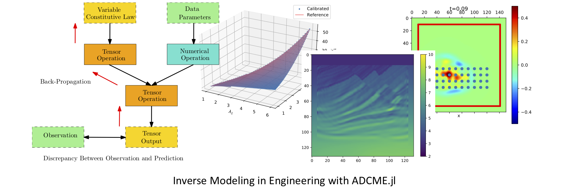
The ADCME library (Automatic Differentiation Library for Computational and Mathematical Engineering) aims at general and scalable inverse modeling in scientific computing with gradient-based optimization techniques. It is built on the deep learning framework, graph-mode TensorFlow, which provides the automatic differentiation and parallel computing backend. The dataflow model adopted by the framework makes it suitable for high performance computing and inverse modeling in scientific computing. The design principles and methodologies are summarized in the slides.
Check out more about slides and videos on ADCME!
| Install ADCME and Get Started (Windows, Mac, and Linux) | Scientific Machine Learning for Inverse Modeling | Solving Inverse Modeling Problems with ADCME | ...more on ADCME Youtube Channel! |
|---|---|---|---|
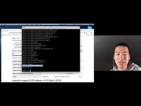 | 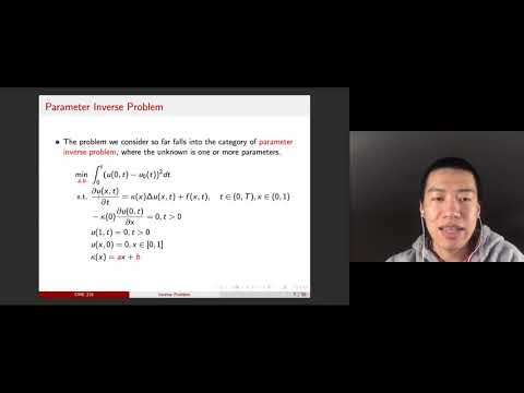 |  |  |
Several features of the library are
- MATLAB-style Syntax. Write
A*Bfor matrix production instead oftf.matmul(A,B). - Custom Operators. Implement operators in C/C++ for performance critical parts; incorporate legacy code or specially designed C/C++ code in
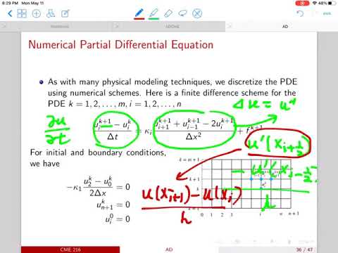
ADCME; automatic differentiation through implicit schemes and iterative solvers. - Numerical Scheme. Easy to implement numerical schemes for solving PDEs.
- Physics Constrained Learning. Embed neural network into PDEs and solve with any numerical schemes, including implicit and iterative schemes.
- Static Graphs. Compilation time computational graph optimization; automatic parallelism for your simulation codes.
- Parallel Computing. Concurrent execution and model/data parallel distributed optimization.
- Custom Optimizers. Large scale constrained optimization? Use
CustomOptimizerto integrate your favorite optimizer. Try out prebuilt Ipopt and NLopt optimizers. - Sparse Linear Algebra. Sparse linear algebra library tailored for scientific computing.
- Inverse Modeling. Many inverse modeling algorithms have been developed and implemented in ADCME, with wide applications in solid mechanics, fluid dynamics, geophysics, and stochastic processes.
 Finite Element Method. Get AdFem.jl today for finite element simulation and inverse modeling!
Start building your forward and inverse modeling using ADCME today!
| Documentation | Tutorial | Applications |
|---|---|---|
Graph-mode TensorFlow for High Performance Scientific Computing
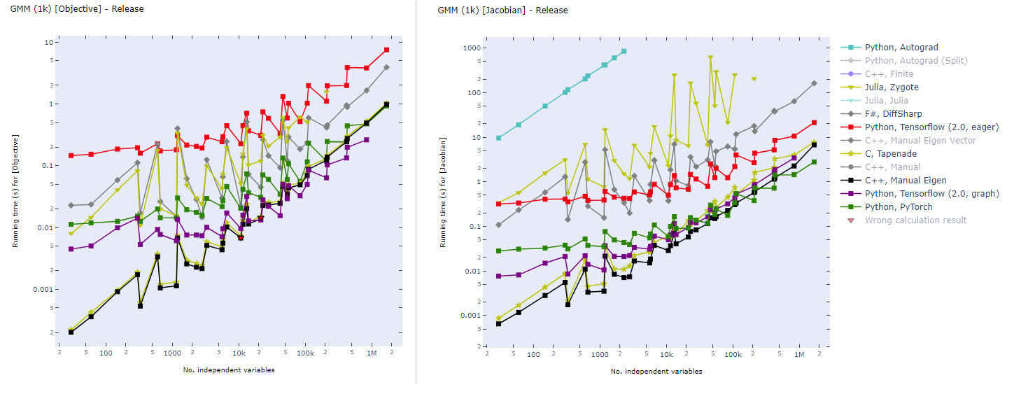
Static computational graph (graph-mode AD) enables compilation time optimization. Below is a benchmark of common AD software from here. In inverse modeling, we usually have a scalar-valued objective function, so the left panel is most relevant for ADCME.
Installation
- Install Julia.
🎉 Support Matrix
| Julia≧1.3 | GPU | Custom Operator | |
|---|---|---|---|
| Linux | ✔ | ✔ | ✔ |
| MacOS | ✔ | ✕ | ✔ |
| Windows | ✔ | ✔ | ✔ |
- Install
ADCME
using Pkg
Pkg.add("ADCME")
❗ FOR WINDOWS USERS: See the instruction or the video for installation details.
❗ FOR MACOS USERS: See this troubleshooting list for potential installation and compilation problems on Mac.
- (Optional) Test
ADCME.jl
using Pkg
Pkg.test("ADCME")
See Troubleshooting if you encounter any compilation problems.
- (Optional) To enable GPU support, make sure
nvccis available from your environment (e.g., typenvccin your shell and you should get the location of the executable binary file), and then type
ENV["GPU"] = 1
Pkg.build("ADCME")
You can check the status with using ADCME; gpu_info().
- (Optional) Check the health of your installed ADCME and install missing dependencies or fixing incorrect paths.
using ADCME
doctor()
For manual installation without access to the internet, see here.
Tutorial
Here we present three inverse problem examples. The first one is a parameter estimation problem, the second one is a function inverse problem where the unknown function does not depend on the state variables, and the third one is also a function inverse problem, but the unknown function depends on the state variables.
Parameter Inverse Problem
Consider solving the following problem

where

Assume that we have observed u(0.5)=1, we want to estimate b. In this case, he true value should be b=1.
using LinearAlgebra
using ADCME

n = 101 # number of grid nodes in [0,1]
h = 1/(n-1)
x = LinRange(0,1,n)[2:end-1]

b = Variable(10.0) # we use Variable keyword to mark the unknowns
A = diagm(0=>2/h^2*ones(n-2), -1=>-1/h^2*ones(n-3), 1=>-1/h^2*ones(n-3))
B = b*A + I  # I stands for the identity matrix
f = @. 4*(2 + x - x^2)
u = B\f # solve the equation using built-in linear solver
ue = u[div(n+1,2)] # extract values at x=0.5

loss = (ue-1.0)^2

# Optimization
sess = Session(); init(sess)
BFGS!(sess, loss)

println("Estimated b = ", run(sess, b))
Expected output
Estimated b = 0.9995582304494237
The gradients can be obtained very easily. For example, if we want the gradients of loss with respect to b, the following code will create a Tensor for the gradient
julia> gradients(loss, b)
PyObject <tf.Tensor 'gradients_1/Mul_grad/Reshape:0' shape=() dtype=float64>
Function Inverse Problem: Full Field Data
Consider a nonlinear PDE,

where

Here f(x) can be computed from an analytical solution

In this problem, we are given the full field data of u(x) (the discrete value of u(x) is given on a very fine grid) and want to estimate the nonparametric function b(u). We approximate b(u) using a neural network and use the residual minimization method to find the optimal weights and biases of the neural network. The minimization problem is given by

using LinearAlgebra
using ADCME
using PyPlot

n = 101
h = 1/(n-1)
x = LinRange(0,1,n)|>collect

u = sin.(π*x)
f = @. (1+u^2)/(1+2u^2) * π^2 * u + u
# `fc` is short for fully connected neural network.
# Here we create a neural network with 2 hidden layers, and 20 neuron per layer.
# The default activation function is tanh.
b = squeeze(fc(u[2:end-1], [20,20,1]))

residual = -b.*(u[3:end]+u[1:end-2]-2u[2:end-1])/h^2 + u[2:end-1] - f[2:end-1]
loss = sum(residual^2)

sess = Session(); init(sess)
BFGS!(sess, loss)

plot(x, (@. (1+x^2)/(1+2*x^2)), label="Reference")
plot(u[2:end-1], run(sess, b), "o", markersize=5., label="Estimated")
legend(); xlabel("\$u\$"); ylabel("\$b(u)\$"); grid("on")
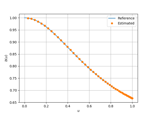
Here we show the estimated coefficient function and the reference one:
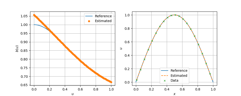
Function Inverse Problem: Sparse Data
Now we consider the same problem as above, but only consider we have access to sparse observations. We assume that on the grid only the values of u(x) on every other 5th grid point are observable. We use the physics constrained learning technique and train a neural network surrogate for b(u) by minimizing

Here uᶿ is the solution to the PDE with

We add 1 to the neural network to ensure the initial guess does not result in a singular Jacobian matrix in the Newton Raphson solver.
using LinearAlgebra
using ADCME
using PyPlot

n = 101
h = 1/(n-1)
x = LinRange(0,1,n)|>collect

u = sin.(π*x)
f = @. (1+u^2)/(1+2u^2) * π^2 * u + u

# we use a Newton Raphson solver to solve the nonlinear PDE problem
function residual_and_jac(θ, x)
    nn = squeeze(fc(reshape(x,:,1), [20,20,1], θ)) + 1.0
    u_full = vector(2:n-1, x, n)
    res = -nn.*(u_full[3:end]+u_full[1:end-2]-2u_full[2:end-1])/h^2 + u_full[2:end-1] - f[2:end-1]
    J = gradients(res, x)
    res, J
end
θ = Variable(fc_init([1,20,20,1]))
ADCME.options.newton_raphson.rtol = 1e-4 # relative tolerance
ADCME.options.newton_raphson.tol = 1e-4 # absolute tolerance
ADCME.options.newton_raphson.verbose = true # print details in newton_raphson
u_est = newton_raphson_with_grad(residual_and_jac, constant(zeros(n-2)),θ)
residual = u_est[1:5:end] - u[2:end-1][1:5:end]
loss = sum(residual^2)

b = squeeze(fc(reshape(x,:,1), [20,20,1], θ)) + 1.0
sess = Session(); init(sess)
BFGS!(sess, loss)

figure(figsize=(10,4))
subplot(121)
plot(x, (@. (1+x^2)/(1+2*x^2)), label="Reference")
plot(x, run(sess, b), "o", markersize=5., label="Estimated")
legend(); xlabel("\$u\$"); ylabel("\$b(u)\$"); grid("on")
subplot(122)
plot(x, (@. sin(π*x)), label="Reference")
plot(x[2:end-1], run(sess, u_est), "--", label="Estimated")
plot(x[2:end-1][1:5:end], run(sess, u_est)[1:5:end], "x", markersize=5., label="Data")
legend(); xlabel("\$x\$"); ylabel("\$u\$"); grid("on")
We show the reconstructed b(u) and the solution u computed from b(u). We see that even though the neural network model fits the data very well, b(u) is not the same as the true one. This problem is ubiquitous in inverse modeling, where the unknown may not be unique.
See Applications for more inverse modeling techniques and examples.
Under the Hood: Computational Graph
A static computational graph is automatic constructed for your implementation. The computational graph guides the runtime execution, saves intermediate results, and records data flows dependencies for automatic differentiation. Here we show the computational graph in the parameter inverse problem:
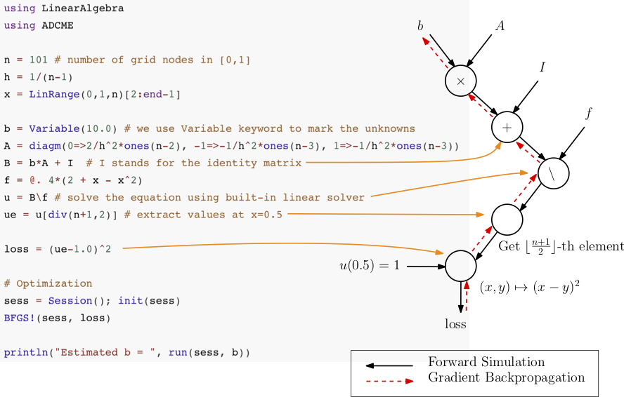
See a detailed tutorial, or a full documentation.
Featured Applications
| Constitutive Modeling | Seismic Inversion | Coupled Two-Phase Flow and Time-lapse FWI | Calibrating Jump Diffusion |
|---|---|---|---|
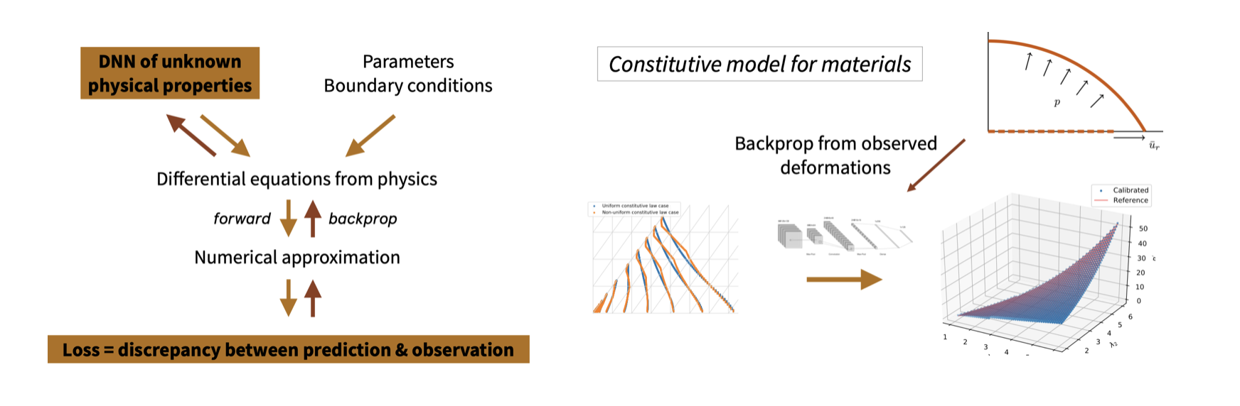 |  | 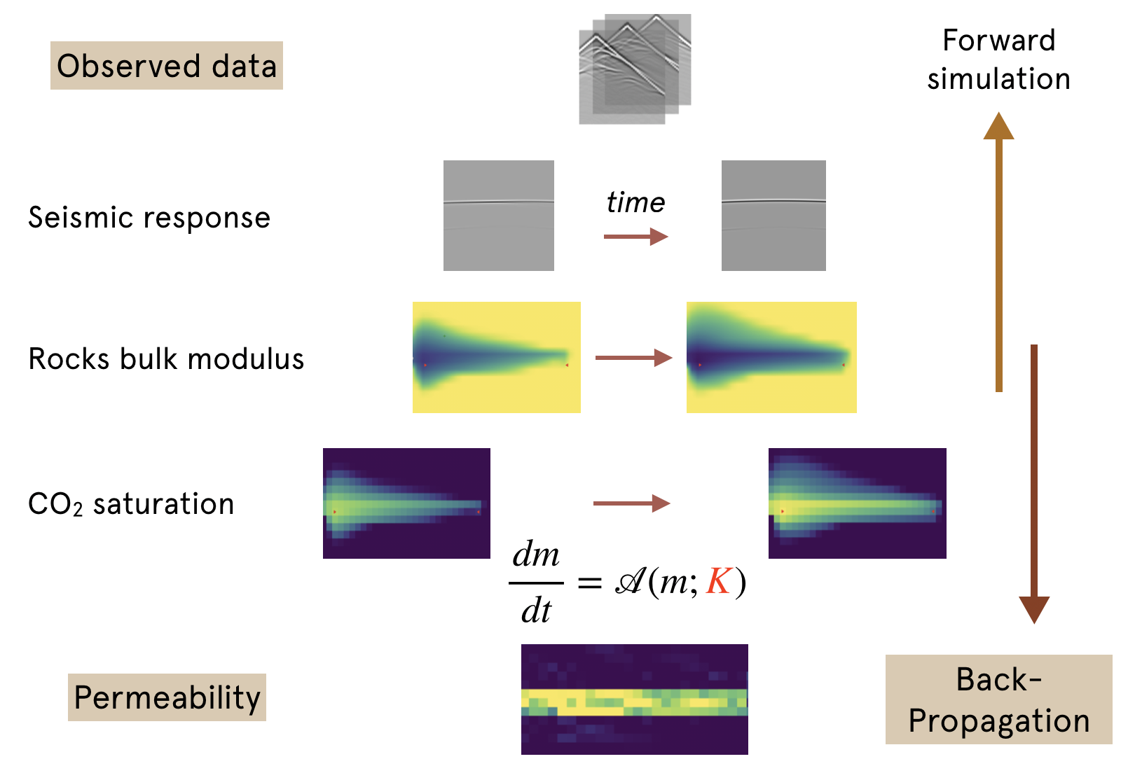 | 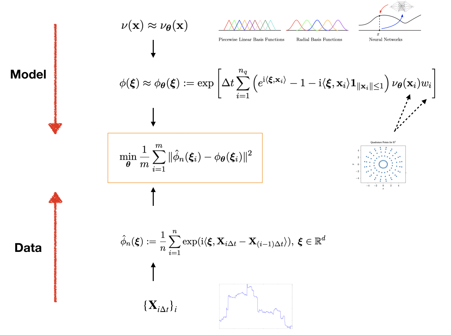 |
Here are some research papers using ADCME:
Li, Dongzhuo, Kailai Xu, Jerry M. Harris, and Eric Darve. "Coupled Time‐Lapse Full‐Waveform Inversion for Subsurface Flow Problems Using Intrusive Automatic Differentiation." Water Resources Research 56, no. 8 (2020): e2019WR027032.
Xu, Kailai, Alexandre M. Tartakovsky, Jeff Burghardt, and Eric Darve. "Inverse Modeling of Viscoelasticity Materials using Physics Constrained Learning." arXiv preprint arXiv:2005.04384 (2020).
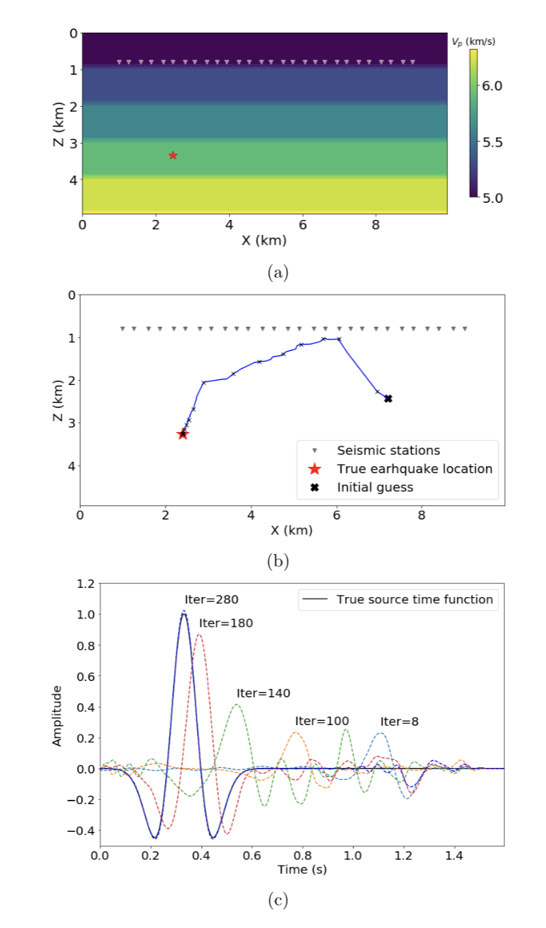
Zhu, Weiqiang, Kailai Xu, Eric Darve, and Gregory C. Beroza. "A General Approach to Seismic Inversion with Automatic Differentiation." arXiv preprint arXiv:2003.06027 (2020).
Xu, K. and Darve, E., 2019. Adversarial Numerical Analysis for Inverse Problems. arXiv preprint arXiv:1910.06936.
Xu, Kailai, Weiqiang Zhu, and Eric Darve. "Distributed Machine Learning for Computational Engineering using MPI." arXiv preprint arXiv:2011.01349 (2020).
Xu, Kailai, and Eric Darve. "Physics constrained learning for data-driven inverse modeling from sparse observations." arXiv preprint arXiv:2002.10521 (2020).
Xu, Kailai, Daniel Z. Huang, and Eric Darve. "Learning constitutive relations using symmetric positive definite neural networks." arXiv preprint arXiv:2004.00265 (2020).
Xu, Kailai, and Eric Darve. "The neural network approach to inverse problems in differential equations." arXiv preprint arXiv:1901.07758 (2019).
Huang, D.Z., Xu, K., Farhat, C. and Darve, E., 2019. Predictive modeling with learned constitutive laws from indirect observations. arXiv preprint arXiv:1905.12530.
Domain specific software based on ADCME
ADSeismic.jl: Inverse Problems in Earthquake Location/Source-Time Function, FWI, Rupture Process
FwiFlow.jl: Seismic Inversion, Two-phase Flow, Coupled seismic and flow equations
AdFem.jl: Inverse Modeling with the Finite Element Method
LICENSE
ADCME.jl is released under MIT License. See License for details.