![]()
![]()
AcousticRayTracers
RaySolver is a differentiable 2½D Gaussian beam tracer for use with UnderwaterAcoustics.jl.
It is similar to Bellhop, but fully written in Julia to be compatible with automatic differentiation
tool such as ForwardDiff, ReverseDiff and Zygote, and other tools including Turing, Measurements, etc.
NOTE: The RaySolver model is experimental and being actively developed, and should be considered as a beta release at present. Feedback and bug reports are welcome.
Installation
julia> # press ]
pkg> add UnderwaterAcoustics
pkg> add AcousticRayTracers
pkg> # press BACKSPACE
julia> using UnderwaterAcoustics
julia> using AcousticRayTracers
julia> models()
2-element Vector{Any}:
 PekerisRayModel
 RaySolver
Usage
The propagation modeling API is detailed in the UnderwaterAcoustics documentation.
We assume that the reader is familiar with it. This documentation only provides guidance on specific use of RaySolver propagation model.
Additional options available with RaySolver:
nbeams-- number of beams used for ray tracing (default: auto)minangle-- minimum beam angle in radians (default: -80°)maxangle-- maximum beam angle in radians (default: 80°)ds-- ray trace step size in meters (default: 1.0)atol-- absolute tolerance of differential equation solver (default: 1e-4)rugocity-- measure of small-scale variations of surfaces (default: 1.5)athreshold-- relative amplitude threshold below which rays are dropped (default: 1e-5)solver-- differential equation solver (default: auto)solvertol-- differential equation solver tolerance (default: 1e-4)
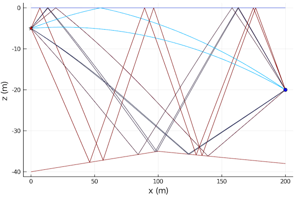
Example:
using UnderwaterAcoustics
using AcousticRayTracers
using Plots

env = UnderwaterEnvironment(
  seasurface = SeaState2,
  seabed = SandyClay,
  ssp = SampledSSP(0.0:20.0:40.0, [1540.0, 1510.0, 1510.0], :linear),
  bathymetry = SampledDepth(0.0:100.0:200.0, [40.0, 35.0, 38.0], :linear)
)
pm = RaySolver(env; nbeams=1000)
tx = AcousticSource(0.0, -5.0, 1000.0)
rx = AcousticReceiver(200.0, -20.0)
r = eigenrays(pm, tx, rx)
plot(env; sources=[tx], receivers=[rx], rays=r)
For more information on how to use the propagation models, see Propagation modeling toolkit.