DataFlowTasks.jl

DataFlowTasks.jl is a Julia package dedicated to parallel programming on multi-core shared memory CPUs. From user annotations (READ, WRITE, READWRITE) on program data, DataFlowTasks.jl automatically infers dependencies between parallel tasks.

This README is also available in notebook form:

Installation

using Pkg
Pkd.add("https://github.com/maltezfaria/DataFlowTasks.jl.git")

Basic Usage

This package defines a @dspawn macro which behaves very much like Threads.@spawn, except that it allows the user to specify explicit data dependencies for the spawned Task. This information is then used to automatically infer task dependencies by constructing and analyzing a directed acyclic graph based on how tasks access the underlying data. The premise is that it is sometimes simpler to specify how tasks depend on data than to specify how tasks depend on each other.

When creating a Task using @dspawn, the following annotations can be used to declare how the Task accesses the data:

• read-only: @R or @READ
• write-only: @W or @WRITE
• read-write: @RW or @READWRITE

An @R(A) annotation for example implies that A will be accessed in read-only mode by the task.

Let's look at a simple example:

using DataFlowTasks
A = Vector{Float64}(undef, 4)
result = let
    @dspawn fill!(@W(A), 0)           # task 1: accesses everything
    @dspawn @RW(view(A, 1:2)) .+= 2   # task 2: modifies the first half
    @dspawn @RW(view(A, 3:4)) .+= 3   # task 3: modifies the second half
    @dspawn @R(A)                     # task 4: get the result
end
fetch(result)

From annotations describing task-data dependencies, DataFlowTasks.jl infers dependencies between tasks. Internally, this set of dependencies is represented as a Directed Acyclic Graph. All the data needed to reconstruct the DAG (as well as the parallalel traces) can be collected using the @log macro:

log_info = DataFlowTasks.@log let
    @dspawn fill!(@W(A), 0)             label="write whole"
    @dspawn @RW(view(A, 1:2)) .+= 2     label="write 1:2"
    @dspawn @RW(view(A, 3:4)) .+= 3     label="write 3:4"
    res = @dspawn @R(A)                 label="read whole"
    fetch(res)
end

And the DAG can be visualized using GraphViz:

DataFlowTasks.stack_weakdeps_env!() # Set up a stacked environment so that weak dependencies such as GraphViz can be loaded. More about that hereafter.
using GraphViz # triggers additional code loading, powered by weak dependencies (julia >= 1.9)
dag = GraphViz.Graph(log_info)

In the example above, the tasks write 1:2 and write 3:4 access different parts of the array A and are therefore independent, as shown in the DAG.

Example : Parallel Cholesky Factorization

As a less contrived example, we illustrate below the use of DataFlowTasks to parallelize a tiled Cholesky factorization. The implementation shown here is delibarately made as simple as possible.

The Cholesky factorization algorithm takes a symmetric positive definite matrix A and finds a lower triangular matrix L such that A = LLᵀ. The tiled version of this algorithm decomposes the matrix A into tiles (of even sizes, in this simplified version). At each step of the algorithm, we do a Cholesky factorization on the diagonal tile, use a triangular solve to update all of the tiles at the right of the diagonal tile, and finally update all the tiles of the submatrix with a Schur complement.

If we have a matrix A decomposed in n x n tiles, then the algorithm will have n steps. The i-th step (with i ∈ [1:n]) will perform

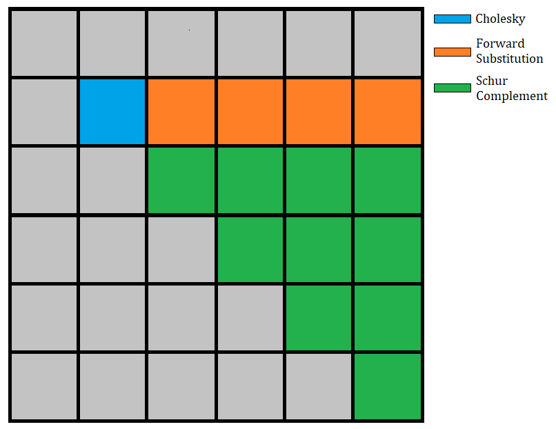
• 1 Cholesky factorization of the (i,i) block,
• (i-1) triangular solves (one for each block in the i-th row),
• i*(i-1)/2 matrix multiplications to update the submatrix.

The following image illustrates the 2nd step of the algorithm:

A sequential tiled factorization algorithm can be implemented as:

using LinearAlgebra

tilerange(ti, ts) = (ti-1)*ts+1:ti*ts

function cholesky_tiled!(A, ts)
    m = size(A, 1); @assert m==size(A, 2)
    m%ts != 0 && error("Tilesize doesn't fit the matrix")
    n = m÷ts  # number of tiles in each dimension

    T = [view(A, tilerange(i, ts), tilerange(j, ts)) for i in 1:n, j in 1:n]

    for i in 1:n
        # Diagonal Cholesky serial factorization
        cholesky!(T[i,i])

        # Left blocks update
        U = UpperTriangular(T[i,i])
        for j in i+1:n
            ldiv!(U', T[i,j])
        end

        # Submatrix update
        for j in i+1:n
            for k in j:n
                mul!(T[j,k], T[i,j]', T[i,k], -1, 1)
            end
        end
    end

    # Construct the factorized object
    return Cholesky(A, 'U', zero(LinearAlgebra.BlasInt))
end

Parallelizing the code with DataFlowTasks.jl is as easy as wrapping function calls within @dspawn, and adding annotations describing data access modes:

using DataFlowTasks

function cholesky_dft!(A, ts)
    m = size(A, 1); @assert m==size(A, 2)
    m%ts != 0 && error("Tilesize doesn't fit the matrix")
    n = m÷ts  # number of tiles in each dimension

    T = [view(A, tilerange(i, ts), tilerange(j, ts)) for i in 1:n, j in 1:n]

    for i in 1:n
        # Diagonal Cholesky serial factorization
        @dspawn cholesky!(@RW(T[i,i])) label="chol ($i,$i)"

        # Left blocks update
        U = UpperTriangular(T[i,i])
        for j in i+1:n
            @dspawn ldiv!(@R(U)', @RW(T[i,j])) label="ldiv ($i,$j)"
        end

        # Submatrix update
        for j in i+1:n
            for k in j:n
                @dspawn mul!(@RW(T[j,k]), @R(T[i,j])', @R(T[i,k]), -1, 1) label="schur ($j,$k)"
            end
        end
    end

    # Construct the factorized object
    r = @dspawn Cholesky(@R(A), 'U', zero(LinearAlgebra.BlasInt)) label="result"
    return fetch(r)
end

(Also note how extra annotations were added in the code, in order to attach meaningful labels to the tasks. These will later be useful to interpret the output of debugging & profiling tools.)

The code below shows how to use this cholesky_tiled! function, as well as how to profile the program and get information about how tasks were scheduled:

# DataFlowTasks environment setup

# Context
n  = 2048
ts = 512
A = rand(n, n)
A = (A + adjoint(A))/2
A = A + n*I;

# First run to trigger compilation
F = cholesky_dft!(copy(A), ts)

# Check results
err = norm(F.L*F.U-A,Inf)/max(norm(A),norm(F.L*F.U))

Debugging and Profiling

DataFlowTasks comes with debugging and profiling tools that help understanding how task dependencies were inferred, and how tasks were scheduled during execution.

As usual when profiling code, it is recommended to start from a state where all code has already been compiled, and all previous profiling information has been discarded:

# Manually call GC to avoid noise from previous runs
GC.gc()

# Profile the code and return a `LogInfo` object:
log_info = DataFlowTasks.@log cholesky_dft!(A ,ts);

Visualizing the DAG can be helpful. When debugging, this representation of dependencies between tasks as inferred by DataFlowTasks can help identify missing or erroneous data dependency annotations. When profiling, identifying the critical path (plotted in red in the DAG) can help understand the performances of the implementation.

In this more complex example, we can see how quickly the DAG complexity increases (even though the test case only has 4x4 blocks here):

dag = GraphViz.Graph(log_info)

The LogInfo object also contains all the data needed to profile the parallel application. A summary of the profiling information can be displayed in the REPL using the DataFlowTasks.describe function:

DataFlowTasks.describe(log_info; categories=["chol", "ldiv", "schur"])

but it is often more convenient to see this information in a graphical way. The parallel trace plot shows a timeline of the tasks execution on available threads. It helps in understanding how tasks were scheduled. The same window also carries other general information allowing to better understand the performance limiting factors:

using CairoMakie # or GLMakie in order to have more interactivity
trace = plot(log_info; categories=["chol", "ldiv", "schur"])

We see here that the execution time is bounded by the length of the critical path: with this block size and matrix size, the algorithm does not expose enough parallelism to occupy all threads without waiting periods.

We'll cover in detail the usage and possibilities of the visualization in the documentation.

Note that the debugging & profiling tools need additional dependencies such as Makie and GraphViz, which are only meant to be used interactively during the development process. These packages are therefore only considered as optional dependencies; assuming they are available in your work environment, calling e.g. using GraphViz will load some additional code from DataFlowTasks. If these dependencies are not directly available in the current environment stack, DataFlowTasks.stack_weakdeps_env!() can be called to push to the loading stack a new environment in which these optional dependencies are available.

Going further: examples and performance

The online documentation contains a variety of examples and benchmarks of applications where DataFlowTasks can be used to parallelize code. These include:

• Cholesky factorization
• Image filters
• Longest common subsequence
• Merge sort

Each example comes with a notebook version, which can be downloaded and run locally: give it a try, and if DataFlowTasks is useful to you, please consider submitting your own example application!

This page was generated using Literate.jl.