AsynchronousIterativeAlgorithms.jl

🧮 AsynchronousIterativeAlgorithms.jl handles the distributed asynchronous communications, so you can focus on designing your algorithm.

💽 It also offers a convenient way to manage the distribution of your problem's data across multiple processes or remote machines.

Installation

You can install AsynchronousIterativeAlgorithms by typing

julia> ] add AsynchronousIterativeAlgorithms

Quick start

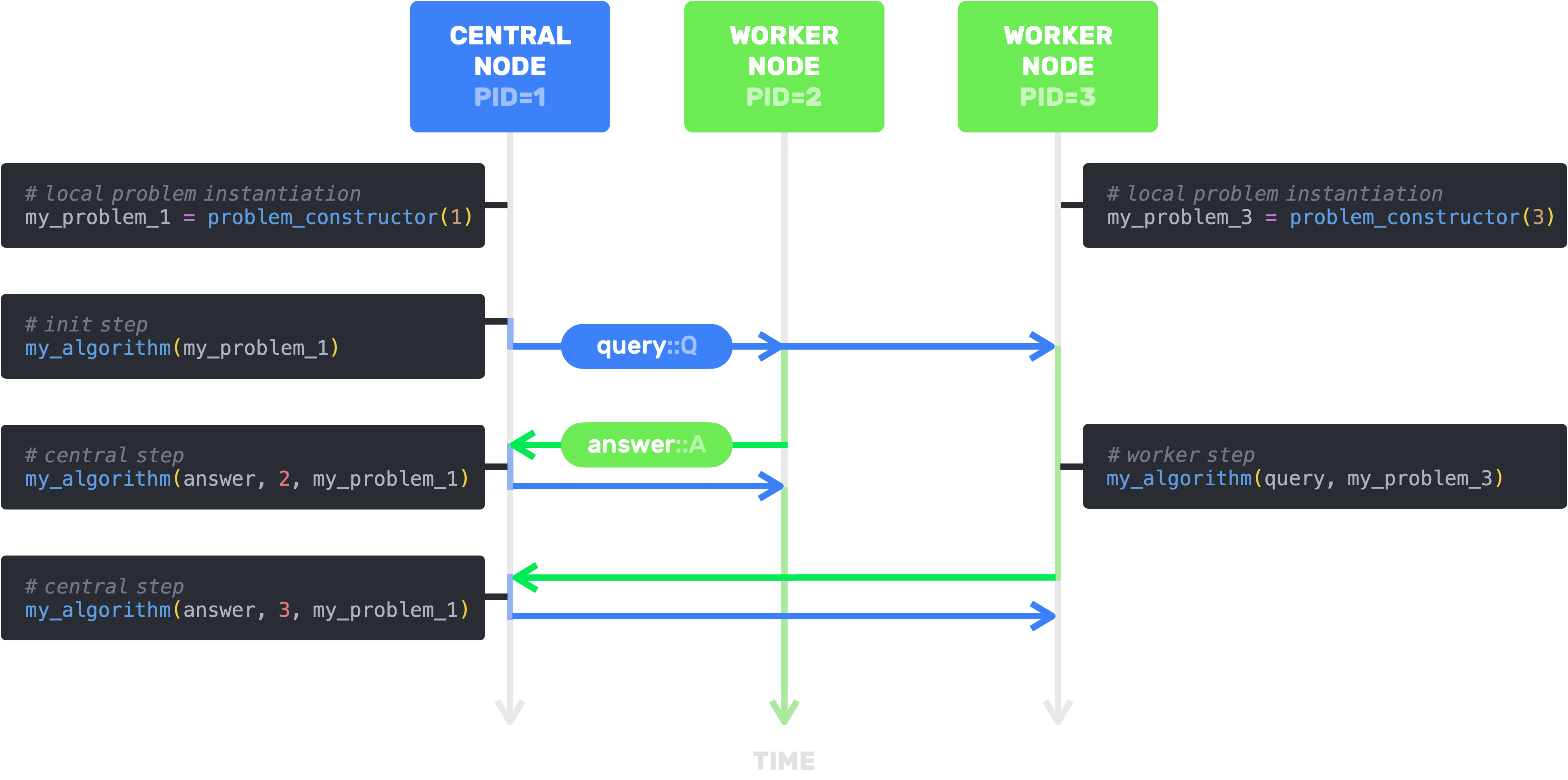
Say you want to implement a distributed version of Stochastic Gradient Descent (SGD). You'll need to define:

• an algorithm structure subtyping AbstractAlgorithm{Q,A}
• the initialization step where you compute the first iteration
• the worker step performed by the workers when they receive a query q::Q from the central node
• the asynchronous central step performed by the central node when it receives an answer a::A from a worker

Let's first of all set up our distributed environment.

# Launch multiple processes (or remote machines)
using Distributed; addprocs(5)

# Instantiate and precompile environment in all processes
@everywhere (using Pkg; Pkg.activate(@__DIR__); Pkg.instantiate(); Pkg.precompile())

# You can now use AsynchronousIterativeAlgorithms
@everywhere (using AsynchronousIterativeAlgorithms; const AIA = AsynchronousIterativeAlgorithms)

Now to the implementation.

# define on all processes
@everywhere begin
    # algorithm
    mutable struct SGD<:AbstractAlgorithm{Vector{Float64},Vector{Float64}}
        stepsize::Float64
        previous_q::Vector{Float64} # previous query
        SGD(stepsize::Float64) = new(stepsize, Float64[])
    end

    # initialisation step 
    function (sgd::SGD)(problem::Any)
        sgd.previous_q = rand(problem.n)
    end

    # worker step
    function (sgd::SGD)(q::Vector{Float64}, problem::Any) 
        sgd.stepsize * problem.∇f(q, rand(1:problem.m))
    end

    # asynchronous central step
    function (sgd::SGD)(a::Vector{Float64}, worker::Int64, problem::Any) 
        sgd.previous_q -= a
    end
end

Now let's test our algorithm on a linear regression problem with mean squared error loss (LRMSE). This problem must be compatible with your algorithm. In this example, it means providing attributes n and m (dimension of the regressor and number of points), and the method ∇f(x::Vector{Float64}, i::Int64) (gradient of the linear regression loss on the ith data point)

@everywhere begin
    struct LRMSE
        A::Union{Matrix{Float64}, Nothing}
        b::Union{Vector{Float64}, Nothing}
        n::Int64
        m::Int64
        L::Float64 # Lipschitz constant of f
        ∇f::Function
    end

    function LRMSE(A::Matrix{Float64}, b::Vector{Float64})
        m, n = size(A)
        L = maximum(A'*A)
        ∇f(x) = A' * (A * x - b) / n
        ∇f(x,i) = A[i,:] * (A[i,:]' * x - b[i])
        LRMSE(A, b, n, m, L, ∇f)
    end
end

We're almost ready to start the algorithm...

# Provide the stopping criteria 
stopat = (iteration=1000, time=42.)

# Instanciate your algorithm 
sgd = SGD(0.01)

# Create a function that returns an instance of your problem for a given pid 
problem_constructor = (pid) -> LRMSE(rand(42,10),rand(42))

# And you can [start](@ref)!
history = start(sgd, problem_constructor, stopat);