Tutorial

Ready-to-run scripts for the functionalities introduced here can be found in the examples directory of the repo.

Creating a bacterium

Bacteria are represented by custom types, that must be subtypes of the AbstractAgent type implemented by Agents.jl.

AbstractMicrobe{D} <: AbstractAgent where {D<:Integer}
YourMicrobeType{D} <: AbstractMicrobe{D}

By default, Bactos.jl provides a basic Microbe type, that is usually sufficient for the simplest types of simulations.

Microbe{D} <: AbstractMicrobe{D}

In order to create a Microbe living in a one-dimensional space we can just call

Microbe{1}(id=0)

It is required to pass a value to the id argument (this behavior might change in the future). All the other parameters will be given default values (as described in the type docstring) if not assigned explicitly.

Similarly, for bacteria living in two or three dimensions we can use

Microbe{2}(id=0)
Microbe{3}(id=0)

Custom parameters can be set via kwargs:

Microbe{3}(
    id = 0,
    pos = (300.0, 0.0, 0.0),
    motility = RunTumble(speed = Normal(40.0, 4.0)),
    vel = rand_vel(3) .* 40.0,
    turn_rate = 1.5,
    state = 0.0,
    rotational_diffusivity = 0.035,
    radius = 0.5
)

Creating a model

BacteriaBasedModel provides a fast way to initialise an AgentBasedModel (from Agents.jl) via the initialise_model function, using a typical procedure. If higher levels of customization are needed, the model will need to be created by hand.

initialise_model(;
    microbes,
    timestep,
    extent, spacing = extent/20, periodic = true,
    random_positions = true,
    model_properties = Dict(),
)

We can now generate a population of microbes and, after choosing an integration timestep and a domain size, we initialise our model, placing the microbes at random locations in the domain.

microbes = [Microbe{3}(id=i) for i in 1:10]
timestep = 0.1
extent = 100.0
model = initialise_model(;
    microbes = microbes,
    timestep = timestep,
    extent = extent
)

AgentBasedModel with 10 agents of type Microbe
 space: periodic continuous space with (100.0, 100.0, 100.0) extent and spacing=5.0
 scheduler: fastest
 properties: timestep

Random walks

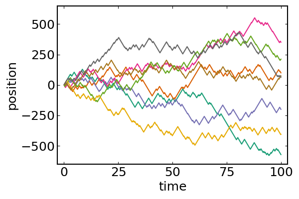
Now we can already generate random walks. The setup follows previous sections.

timestep = 0.1
extent = 1e6 # just a large value to stay away from boundaries
nmicrobes = 8
# initialise all microbes at same position
microbes = [Microbe{1}(id=i, pos=(L/2,)) for i in 1:nmicrobes]

model = initialise_model(;
    microbes,
    timestep,
    extent, periodic = false,
    random_positions = false
)

Now we need to define the adata variable to choose what observables we want to track, throughout the simulation, for each agent in the system. In our case, only the position field

adata = [:pos]

Now we can run the simulation; the microbe_step! function will take care of the stepping and reorientations according to the properties of each microbe:

nsteps = 1000
adf, = run!(model, microbe_step!, nsteps; adata)

x = first.(vectorize_adf_measurement(adf, :pos))'
plot(
    (0:nsteps).*dt, x,
    legend = false,
    xlab = "time",
    ylab = "position"
)

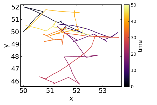
Similarly for a two-dimensional random walk, using run-reverse-flick motility and non-zero rotational diffusion:

dt = 0.1
L = 1000.0
nmicrobes = 1
microbes = [
    Microbe{2}(
        id=i, pos=(L/2,L/2),
        motility=RunReverseFlick(),
        rotational_diffusivity = 0.2,
        ) for i in 1:nmicrobes
]

model = initialise_model(;
    microbes,
    timestep = dt,
    extent, periodic = false,
    random_positions = false,
)

nsteps = 500
adata = [:pos]
adf, = run!(model, microbe_step!, nsteps; adata)

traj = vectorize_adf_measurement(adf, :pos)
x = first.(traj)'
y = last.(traj)'
plot(
    x, y, line_z = (0:nsteps).*dt,
    legend=false,
    xlab = "x", ylab = "y",
    colorbar = true, colorbar_title = "time"
)

Microbes with different motile patterns can also be combined in the same simulation, without extra complications or computational costs:

n = 3
microbes_runtumble = [Microbe{2}(id=i, motility=RunTumble()) for i in 1:n]
microbes_runrev = [Microbe{2}(id=n+i, motility=RunReverse()) for i in 1:n]
microbes_runrevflick = [Microbe{2}(id=2n+1, motility=RunReverseFlick()) for i in 1:n]
microbes = vcat(
    microbes_runtumble, microbes_runrev, microbes_runrevflick
)

Chemotaxis in a linear gradient

We will now reproduce a classical chemotaxis assay: bacteria in a rectangular channel with a linear attractant gradient.

Bactos.jl requires three functions to be defined for the built-in chemotaxis models to work: concentration_field, concentration_gradient, and concentration_time_derivative; all three need to take the two arguments (pos, model). First we need to define our concentration field and its gradient (we don't define its time derivative since it will be held constant). We will use a linear gradient in the x direction. Here we can define also the gradient analytically, in more complex cases it can be evaluated numerically through the finite difference interface.

concentration_field(x,y,C₀,∇C) = C₀ + ∇C*x
function concentration_field(pos, model)
    x, y = pos
    C₀ = model.C₀
    ∇C = model.∇C
    concentration_field(x, y, C₀, ∇C)
end
concentration_gradient(x,y,C₀,∇C) = [∇C, 0.0]
function concentration_gradient(pos, model)
    x, y = pos
    C₀ = model.C₀
    ∇C = model.∇C
    concentration_gradient(x, y, C₀, ∇C)
end

We choose the parameters, initialise the population (with two distinct chemotaxers) with all bacteria to the left of the channel, and setup the model providing the functions for our concentration field to the model_properties dictionary.

timestep = 0.1 # s
Lx, Ly = 1000.0, 500.0 # μm
extent = (Lx, Ly) # μm
periodic = false

n = 50
microbes_brumley = [
    Brumley{2}(id=i, pos=(0,rand()*Ly), chemotactic_precision=1)
    for i in 1:n
]
microbes_brown = [
    BrownBerg{2}(id=n+i, pos=(0,rand()*Ly))
    for i in 1:n
]
microbes = [microbes_brumley; microbes_brown]

C₀ = 0.0 # μM
∇C = 0.01 # μM/μm
model_properties = Dict(
    :concentration_field => concentration_field,
    :concentration_gradient => concentration_gradient,
    :concentration_time_derivative => (_,_) -> 0.0,
    
    :compound_diffusivity => 500.0, # μm²/s
    :C₀ => C₀,
    :∇C => ∇C,
)

model = initialise_model(;
    microbes,
    timestep,
    extent, periodic,
    model_properties,
    random_positions = false
)

Notice that we also defined an extra property compound_diffusivity. This quantity is required by the models of chemotaxis that use sensing noise (such as Brumley, XieNoisy, CelaniNoisy). 500 μm²/s is a typical value for small molecules.

We can run the simulation as usual and extract the trajectories.

adata = [:pos]
nsteps = 1000 # corresponds to 100s
adf, = run!(model, microbe_step!, nsteps; adata)

traj = vectorize_adf_measurement(adf, :pos)
x = first.(traj)'
y = last.(traj)'

Comparing the trajectories for the two bacterial species we witness a chemotactic race (Brumley in blue, BrownBerg in orange).