MetaPhlAn Tutorial with BiobakeryUtils.jl

• 🗒️ This tutorial is meant to be run in parallel with / mirror the official MetaPhlAn v3 tutorial
• ❓️ If you have questions about MetaPhlAn itself, please direct them to the bioBakery help forum
• 🤔 If you have questions about using the MetaPhlAn tools in julia, please open an issue, or start a discussion over on Microbiome.jl!
• 📔 For a function / type reference, jump to the bottom

Installation and setup

If you haven't already, check out the "Getting Started" page to install julia, create an environment,xd and install BiobakeryUtils.jl, and hook up or install the MetaPhlAn v3 command line tools.

This tutorial assumes:

1. You are running julia v1.6 or greater
2. You have activated a julia Project that has BiobakeryUtils.jl installed
3. The metaphlan python package is installed, and accessible from your PATH.

If any of those things aren't true, or you don't know if they're true, go back to "Getting Started" to see if you skipped a step. If you're still confused, please ask (see 3rd bullet point at the top)!

Bowtie2 database

The first time you run metaphlan, it needs to download and unpack the marker database. If you don't care where this goes, don't worry about it - by default it will go into a subdirectory of your conda environment.

If your home folder has limited space, or you want to install it to a particular location (eg a faster drive), you can either pass the kewword argument bowtie2db="/path/to/location" to all metaphlan commands, or set the environment variable METAPHLAN_BOWTIE2_DB.

Input files

Official tutorial link

Some example files you can use to run this tutorial are available from the MetaPhlAn repo, and can be downloaded using the Downloads standard library in julia:

julia> using Downloads: download

julia> base_url = "https://github.com/biobakery/biobakery/raw/master/demos/biobakery_demos/data/metaphlan3/input/";

julia>  files = [
    "SRS014476-Supragingival_plaque.fasta.gz",
    "SRS014494-Posterior_fornix.fasta.gz",
    "SRS014459-Stool.fasta.gz",
    "SRS014464-Anterior_nares.fasta.gz",
    "SRS014470-Tongue_dorsum.fasta.gz",
    "SRS014472-Buccal_mucosa.fasta.gz"
];

julia> for file in files
           download(joinpath(base_url, file), file)
       end

julia> readdir()
9-element Vector{String}:
 "Manifest.toml"
 "Project.toml"
 "SRS014459-Stool.fasta.gz"
 "SRS014464-Anterior_nares.fasta.gz"
 "SRS014470-Tongue_dorsum.fasta.gz"
 "SRS014472-Buccal_mucosa.fasta.gz"
 "SRS014476-Supragingival_plaque.fasta.gz"
 "SRS014494-Posterior_fornix.fasta.gz"

Run a single sample

Official tutorial link

For convenience, this package has the metaphlan() function, which can be used in your julia scripts to build and call the metaphlan command line tool.

For example, rather than call this from the shell:

$ metaphlan SRS014476-Supragingival_plaque.fasta.gz --input_type fasta > SRS014476-Supragingival_plaque_profile.txt

you can instead call this from the julia REPL:

julia> metaphlan("SRS014476-Supragingival_plaque.fasta.gz",
                 "SRS014476-Supragingival_plaque_profile.tsv"; input_type="fasta")

The first time you run this command, metaphlan will download its database and build Bowtie2 indices for aligning marker genes. It may take a while... maybe go for a walk 🙂.

Output files

Official tutorial link

You can now load this profile using metaphlan_profile:

julia> mp = metaphlan_profile("SRS014476-Supragingival_plaque_profile.tsv"; sample="SRS014476")
CommunityProfile{Float64, Taxon, MicrobiomeSample} with 11 features in 1 samples

Feature names:
Bacteria, Actinobacteria, Actinobacteria...Corynebacterium_matruchotii, Rothia_dentocariosa

Sample names:
SRS014476

This generates a CommunityProfile type from Microbiome.jl, which is a matrix-like object with MicrobiomeSamples as column headers, and Taxons as row headers.

The samples can be accessed with samples or samplenames:

julia> samples(mp)
1-element Vector{MicrobiomeSample}:
 MicrobiomeSample("SRS014476", {})

julia> samplenames(mp)
1-element Vector{String}:
 "SRS014476"

Notice that in addition to the sample name ("SRS014476"), there's an additional field - that's a metadata dictionary that we can add values to.

julia> plaque = first(samples(mp))
MicrobiomeSample("SRS014476", {})

julia> set!(plaque, :STSite, "Supragingival Plaque")
MicrobiomeSample("SRS014476", {:STSite = "Supragingival Plaque"})

The taxa (Microbiome.jl uses the generic term "features") can be accessed with features or featurenames:

julia> features(mp)
11-element Vector{Taxon}:
 Taxon("Bacteria", :kingdom)
 Taxon("Actinobacteria", :phylum)
 Taxon("Actinobacteria", :class)
 Taxon("Corynebacteriales", :order)
 Taxon("Micrococcales", :order)
 Taxon("Corynebacteriaceae", :family)
 Taxon("Micrococcaceae", :family)
 Taxon("Corynebacterium", :genus)
 Taxon("Rothia", :genus)
 Taxon("Corynebacterium_matruchotii", :species)
 Taxon("Rothia_dentocariosa", :species)

julia> featurenames(mp)
11-element Vector{String}:
 "Bacteria"
 "Actinobacteria"
 "Actinobacteria"
 "Corynebacteriales"
 "Micrococcales"
 "Corynebacteriaceae"
 "Micrococcaceae"
 "Corynebacterium"
 "Rothia"
 "Corynebacterium_matruchotii"
 "Rothia_dentocariosa"

Run on multiple cores

Official tutorial link

Other keywords can be passed to metaphlan() as well. For example, to speed things up a bit, try nproc=4:

julia> metaphlan("SRS014459-Stool.fasta.gz",
                        "SRS014459-Stool_profile.tsv"; input_type="fasta", nproc=4)
[ Info: Running command: metaphlan SRS014459-Stool.fasta.gz SRS014459-Stool_profile.tsv --input_type fasta --nproc 4
# ... 

Run multiple samples

Official tutorial link

You can use julia to run metaphlan in a loop to do the rest of the files. Here, we find the output path by replacing .fasta.gz with _profile.tsv, then check if it exists already, and continue if it does (&& means "AND" - if isfile(prof) is true, then it will do the thing on the right).

julia> for f in files
           prof = replace(f, ".fasta.gz"=>"_profile.tsv")
           isfile(prof) && continue
           metaphlan(f, prof; input_type="fasta", nproc=4)
       end
┌ Info: Running command: metaphlan SRS014494-Posterior_fornix.fasta.gz SRS014494-Posterior_fornix_profile.tsv --input_type fasta
└ --nproc 4

Merge outputs

Official tutorial link

There are several ways to merge these profiles into one large table. One way is to use merge_metaphlan_tables.py, which has a convenient wrapper, metaphlan_merge:

julia> profiles = filter(f-> contains(f, "profile"), readdir())
6-element Vector{String}:
 "SRS014459-Stool_profile.tsv"
 "SRS014464-Anterior_nares_profile.tsv"
 "SRS014470-Tongue_dorsum_profile.tsv"
 "SRS014472-Buccal_mucosa_profile.tsv"
 "SRS014476-Supragingival_plaque_profile.tsv"
 "SRS014494-Posterior_fornix_profile.tsv"

julia> metaphlan_merge(profiles, "merged_abundance_table.tsv")
Process(`merge_metaphlan_tables.py -o merged_abundance_table.tsv SRS014459-Stool_profile.tsv SRS014464-Anterior_nares_profile.tsv S
RS014470-Tongue_dorsum_profile.tsv SRS014472-Buccal_mucosa_profile.tsv SRS014476-Supragingival_plaque_profile.tsv SRS014494-Posteri
or_fornix_profile.tsv`, ProcessExited(0))

Then, you can load it as a CommunityProfile using metaphlan_profiles():

julia> mps = metaphlan_profiles("merged_abundance_table.tsv"; samplestart=3)
CommunityProfile{Float64, Taxon, MicrobiomeSample} with 62 features in 6 samples

Feature names:
Bacteria, Actinobacteria, Actinobacteria...Moraxella, Moraxella_nonliquefaciens

Sample names:
SRS014494-Posterior_fornix, SRS014476-Supragingival_plaque, SRS014472-Buccal_mucosa...SRS014464-Anterior_nares, SRS014459-Stool

Note, the samplestart=3 argument is necessary because the second column file generated by merge_metaphlan_tables.py contains NCBI taxonomy IDs.

An alternative is to load each individual sample as a CommunityProfile, and then merge them with commjoin:

julia> mps2 = commjoin([metaphlan_profile(p) for p in profiles]...)
CommunityProfile{Float64, Taxon, MicrobiomeSample} with 62 features in 6 samples

Feature names:
Bacteria, Firmicutes, Bacteroidetes...Lactobacillus_crispatus, Lactobacillus_iners

Sample names:
SRS014459-Stool_profile, SRS014464-Anterior_nares_profile, SRS014470-Tongue_dorsum_profile...SRS014476-Supragingival_plaque_profile
, SRS014494-Posterior_fornix_profile

If you'd like that saved to disk, you can use CSV.jl:

julia> using CSV

julia> CSV.write("merged_abundance_table2.tsv", mps2)
"merged_abundance_table2.tsv"

One benefit of doing it the later way is that as we're loading the tables, we can attach some metadata to them. For example:

julia> my_profiles = [] # an empty vector
Any[]

julia> for p in profiles
           file_wo_ext = first(splitext(p))
           (srs, site) = split(file_wo_ext, '-')
           site = replace(site, "_profile"=> "")

           sample = MicrobiomeSample(srs)
           set!(sample, :STSite, site)
           set!(sample, :filename, p)
           push!(my_profiles, metaphlan_profile(p; sample))
       end

julia> mps3 = commjoin(my_profiles...)
CommunityProfile{Float64, Taxon, MicrobiomeSample} with 62 features in 6 samples

Feature names:
Bacteria, Firmicutes, Bacteroidetes...Lactobacillus_crispatus, Lactobacillus_iners

Sample names:
SRS014459, SRS014464, SRS014470...SRS014476, SRS014494



julia> get(mps3)
6-element Vector{NamedTuple{(:sample, :STSite, :filename), Tuple{String, String, String}}}:
 (sample = "SRS014459", STSite = "Stool", filename = "SRS014459-Stool_profile.tsv")
 (sample = "SRS014464", STSite = "Anterior_nares", filename = "SRS014464-Anterior_nares_profile.tsv")
 (sample = "SRS014470", STSite = "Tongue_dorsum", filename = "SRS014470-Tongue_dorsum_profile.tsv")
 (sample = "SRS014472", STSite = "Buccal_mucosa", filename = "SRS014472-Buccal_mucosa_profile.tsv")
 (sample = "SRS014476", STSite = "Supragingival_plaque", filename = "SRS014476-Supragingival_plaque_profile.tsv")
 (sample = "SRS014494", STSite = "Posterior_fornix", filename = "SRS014494-Posterior_fornix_profile.tsv")

See Microbiome.jl docs for more info on metadata and CommunityProfiles)

Analyze Results

Official tutorial link

With the profile loaded, you can use many julia packages to analyze or visualize the results. Inside the CommunityProfile is a sparce matrix, which you can access with abundances. This means that all of julia's powerful statistics and ML libraries are easy to use with your microbiome data.

For more information about indexing and accessing components of the data, see the Microbiome.jl docs

Performing PCoA analysis

To demonstrate this, we'll use a couple of other julia packages to perform and plot a principal coordinates analysis (PCoA): Distances.jl and MulitvariateStats.jl.

(Actually some convenent functions for this are re-exported from Microbiome.jl eg braycurtis and pcoa – this is just meant to show how easy it is to use the underlying data for whatever you like)

You can install these by opening the Pkg REPL (type ']') and using add:

(my_project) pkg> add MultivariateStats Distances
   Resolving package versions...
    Updating `~/my_project/Project.toml`
  [b4f34e82] + Distances v0.10.4
  [6f286f6a] + MultivariateStats v0.8.0
  No Changes to `~/my_project/Manifest.toml`

julia> # type <backspace> to get back to normal REPL

julia> using MultivariateStats

julia> using Distances

Since abundances gives us a normal matrix, we can easily use all the power of other julia packages to do analysis. Here, we'll create a distance matrix use Bray-Curtis dissimilarity, and then do multi dimensional scaling to get our PCoA ordination^[note].

julia> dm = pairwise(BrayCurtis(), abundances(mps3), dims=2) # parwise distances of columns (dimension 2)
6×6 Matrix{Float64}:
 0.0       0.853268  0.662373  0.758712  0.857143  0.758712
 0.853268  0.0       0.845517  0.841645  0.857143  0.845517
 0.662373  0.845517  0.0       0.77874   0.857143  0.787196
 0.758712  0.841645  0.77874   0.0       0.857143  0.461648
 0.857143  0.857143  0.857143  0.857143  0.0       0.857143
 0.758712  0.845517  0.787196  0.461648  0.857143  0.0

julia> pc = fit(MDS, dm, distances=true)
Classical MDS(indim = NaN, outdim = 5)

For plotting, I use Makie, but there are many other options.

(my_project) pkg> add CairoMakie
# ...

julia> using CairoMakie

julia> sites = [m.STSite for m in get(mps3)] # or get(m, :STSite)
6-element Vector{String}:
 "Stool"
 "Anterior_nares"
 "Tongue_dorsum"
 "Buccal_mucosa"
 "Supragingival_plaque"
 "Posterior_fornix"

julia> clrs = [:lightgreen, :cyan, :dodgerblue, :orange, :salmon, :purple]
6-element Vector{Symbol}:
 :lightgreen
 :cyan
 :dodgerblue
 :orange
 :salmon
 :purple

julia> loads = sqrt.(pc.λ)' .* projection(pc) # loadings for pcoa, columns are axes

julia> fig, ax, plt = scatter(loads[:,1], loads[:, 2], color=clrs,
                              axis=(
                                  xlabel="PCoA.1",
                                  ylabel="PCoA.2",
                                  title="Demo PCoA"
                              ))

julia> leg = Legend(fig[1,2], [MarkerElement(color = c, marker=:circle) for c in clrs], sites)
Legend()

julia> fig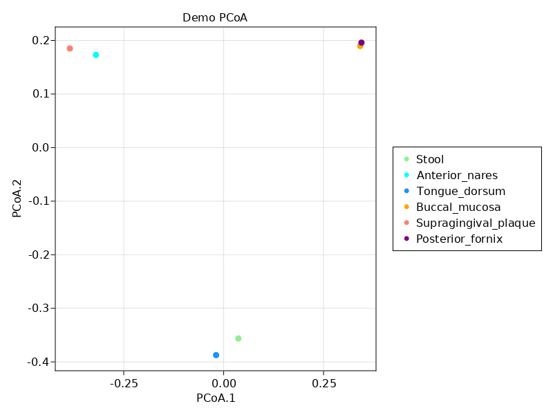

Stacked bar

One more example - let's plot the proportion of different phyla in each sample. First, we'll filter the table to keep only rows that contain phyla. The filter acts on a CommunityProfile by applying the predicate to the features of the profile.

julia> phyl = filter(t-> taxrank(t) == :phylum, mps3)
CommunityProfile{Float64, Taxon, MicrobiomeSample} with 4 features in 6 samples

Feature names:
Firmicutes, Bacteroidetes, Proteobacteria, Actinobacteria

Sample names:
SRS014459, SRS014464, SRS014470...SRS014476, SRS014494

julia> phylumnames = featurenames(phyl)
4-element Vector{String}:
 "Firmicutes"
 "Bacteroidetes"
 "Proteobacteria"
 "Actinobacteria"

julia> fig2 = Figure()

julia> ax2 = Axis(fig2[1,1], title="Phyla in samples", xticks=(1:nsamples(phyl), sites));

julia> ax2.xticklabelrotation = π / 4 # rotations are in radians, type 'π' by doing `\pi<tab>`
0.7853981633974483

julia> y = Float64[]
Float64[]

julia> for sample in samples(phyl)
           abs = abundances(phyl[:, sample])
           abs = abs ./ sum(abs)
           append!(y, abs)
       end

julia> x = repeat(1:nsamples(phyl), inner=nfeatures(phyl))
24-element Vector{Int64}:
 1
 1
 1
 1
 2
 2
 ⋮
 5
 5
 6
 6
 6
 6

julia> sitenums = repeat(1:nfeatures(phyl), outer=nsamples(phyl))
24-element Vector{Int64}:
 1
 2
 3
 4
 1
 2
 ⋮
 3
 4
 1
 2
 3
 4

julia> barplot!(ax2, x, y, stack=sitenums,
               color=sitenums, colormap=:Accent_5)
Combined{Makie.barplot, Tuple{Vector{Point{2, Float32}}}}

julia> leg = Legend(fig2[1,2], [MarkerElement(color = c, marker=:rect) for c in to_colormap(:Accent_5, 4)], phylumnames)
Legend()

julia> fig2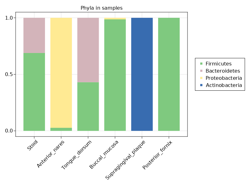

Functions and Types

metaphlan(inputfile, outputfile; kwargs...)

$ metaphlan some.fastq.gz output/some_profile.tsv --input_type fastq --nproc 8

metaphlan("some.fastq.gz", "output/some_profile.tsv"; input_type="fastq", nproc=8)

metaphlan_merge(paths, outputfile; kwargs...)

metaphlan_profile(path::AbstractString, rank::Union{Int, Symbol}=:all; sample::AbstractString=basename(first(splitext(path))))

metaphlan_profiles(path::AbstractString, rank::Union{Int, Symbol}=:all; keepunidentified=false)

metaphlan_profiles(paths::Array{<:AbstractString, 1}, rank::Union{Int, Symbol}=:all)

parsetaxa(taxstring::AbstractString; throw_error=true)

parsetaxon(taxstring::AbstractString, rank::Union{Int, Symbol})