• Postprocessing
• • Using the simulation outputs
  • Plot the final solution
  • biofilm_analyze() - Query Simulation at Specified Times
  • biofilm_movie() - Make movie of biofilm quantities
  • biofilm_sol2csv() - Convert solution to CSV file

Postprocessing

When a simulation completes the solver outputs solution data that can be postprocessed to see additional values and/or plots.

Using the simulation outputs

When a simulation is executed using t,zm,Xt,St,Pb,Sb,Lf,sol = BiofilmSolver(p), which is a line of code within each of the Case files solver will produce all the outputs described below

• t - array of the solution times
• zm - array of the biofilm grid locations at the end of the simulation t[end]
• Xt=Xt(t) - array of the particulate concentrations within the tank as a function of time
• St=St(t) - array of the solute concentrations within the tank as a function of time
• Pb=Pb(z) - array of the particulate volume fractions within the biofilm as a function of location within biofilm at the end of the simulation
• Sb=Sb(z) - array of the solute concentrations within the biofilm as a function of location within biofilm at the end of the simulation
• Lf=Lf(t) - array of the biofilm thickness as a function of time
• sol - entire solution from the ODE solver - contains the time history of all the variables. This variable is difficult to parse but is used by the functions described below.

The output can be analyzed using Julia commands. For example, after running Case1.jl (see Run Biofilm.jl), the maximum solute concentration in the tank could be found

julia> maximum(St)
65.37595010026911

Plot the final solution

The solution can be plotted using the plot recipe biofilm_plot(sol,p), which will produce the standard plots of the simulation. This is useful to make a plot of the solution at the end of the simulation, especially if plots are turned off during the simulation using the optional parameter makePlots=false.

An optional third argument desc can be passed to biofilm_plot, e.g., biofilm_plot(sol,p,"Case A"), which will add "Case A" to the legend labels.

biofilm_plot(sol,p)
biofilm_plot(sol,p,desc)

biofilm_analyze() - Query Simulation at Specified Times

The biofilm_analyze(sol,p,t) function provides a simple way to postprocess data. This function takes in the computed solution sol and parameters p and analyzes the results and the specified time or times t. For example, after running Case1.jl (see Run Biofilm.jl) you could look at the solution at t=0.25 days using

julia> biofilm_analyze(sol,p,0.25)
Analyzing Single Solute and Particulate Case
   Time   |      Bug |   Oxygen | min,max(     Bug) | min,max(  Oxygen) |  Lf [μm] 
    0.250 |      102 |     51.7 |     0.08,    0.08 |     29.1,    51.3 |      545

which displays the tank and biofilm particulates and solutes and biofilm thickness at the requested time. Multiple times can be included in the time parameter. For example to get the values at t=0, 0.25, 0.5, 0.75, 1.0 we can run

julia> biofilm_analyze(sol,p,0:0.25:1)
Analyzing Single Solute and Particulate Case
   Time   |      Bug |   Oxygen | min,max(     Bug) | min,max(  Oxygen) |  Lf [μm] 
    0.000 |       10 |       10 |     0.08,    0.08 |        0,       0 |       10
    0.250 |      102 |     51.7 |     0.08,    0.08 |     29.1,    51.3 |      545
    0.500 |      256 |     2.94 |     0.08,    0.08 |    0.568,    2.87 |      348
    0.750 |      257 |     2.93 |     0.08,    0.08 |    0.745,    2.87 |      312
    1.000 |      257 |     2.93 |     0.08,    0.08 |    0.761,    2.87 |      309

Adding an optional argument makePlot=true, i.e., biofilm_analyze(sol,p,0.25,makePlot=true) will produce a plot of the biofilm quantities at the specified time(s)

julia> biofilm_analyze(sol,p,0.25,makePlot=true)
Analyzing Single Solute and Particulate Case
   Time   |      Bug |   Oxygen | min,max(     Bug) | min,max(  Oxygen) |  Lf [μm] 
    0.250 |      102 |     51.7 |     0.08,    0.08 |     29.1,    51.3 |      545

biofilm_analyze(sol,p,times)
biofilm_analyze(sol,p,times,makePlot=true)

biofilm_movie() - Make movie of biofilm quantities

The particulate and solute concentrations change throughout the simulation, and it is often useful to make movies of how these change over time.

The biofilm_movie(times) function provides a convenient way to make these movies. For example, to post process Case 5 - Phototroph, which has a light that turns on and off throughout each day we could make a movie of the biofilm conditions during the day and during night. To make a movie of every 5 days when the light is on, that is at times=1,5,10,... we can use

julia> biofilm_movie(sol,p,1:5:t[end],filename="phototroph_day.gif",fps=5)

which will analyze each day and combine the results into the movie: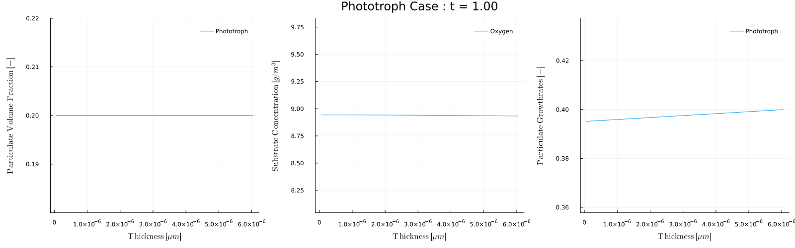

To produce the results every 5th night, that is at times=0.5, 5.5, ... we can use

julia> biofilm_movie(sol,p,0.5:5:t[end],filename="phototroph_night.gif",fps=5)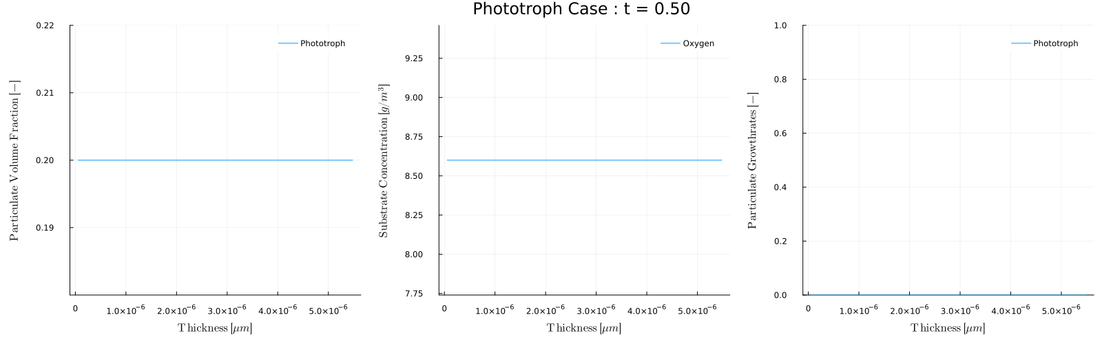

Note that during the day the growth rate is zero and the oxygen concentration is 8.6, which is the inflow concentration Sin. During the day however, the phototroph growth rate is non-zero, and the growth produces oxygen.

biofilm_movie(sol,p,times)
biofilm_movie(sol,p,times,filename="anim.gif", fps=20)

julia> biofilm_movie(sol,p,0:1:10)

julia> biofilm_movie(sol,p,0:1:10,filename="biofilm.gif",fps=10)

biofilm_sol2csv() - Convert solution to CSV file

The function biofilm_sol2csv( sol, p) takes the output of a simulation and writes the results as a CSV file which can be open in a spreadsheet program (e.g., Excel). Each row in the file corresponds to a different output time and the column contains the time, the tank particulate and solute concentrations, biofilm particulate volume fractions and solute concentrations, and finally the biofilm thickness. This function can be useful for users that prefer looking at results in a spreadsheet.

biofilm_sol2csv(sol,p)
biofilm_sol2csv(sol,p; filename)

julia> biofilm_sol2csv(sol,p)
julia> biofilm_sol2csv(sol,p,filename="myfile.csv")