Type_IOP(n::Integer, nc::Integer [, a [; nam="" [; msg=true]]])

BigInt if n is a BigInt or n > nc, otherwise Int; a is an auxiliary second variable.

• nam : function name

• msg : integer-overflow protection (IOP) - warning on activation

Examples:

julia> Type_IOP(1, 1)
Int64

julia> Type_IOP(big(1), 1)
BigInt

julia> Type_IOP(2, 1)
BigInt

julia> Type_IOP(1, 1; nam="test")
Int64

julia> Type_IOP(2, 1, 0; nam="test")
 IOP capture at test(2, 0): output converted to BigInt
BigInt

log10_characteristic(x)

characteristic power-of-10 of the number x

Examples:

log10_characteristic.([3,30,300])
3-element Vector{Int64}:
 0
 1
 2

log10_mantissa(x)

log10 mantissa of the number x

Examples:

log10_mantissa.([3,30,300])
3-element Vector{Float64}:
 0.47712125471966244
 0.4771212547196624
 0.4771212547196626

texp(x::T, a::T, p::Int) where T <: Real

Truncated exponential: Taylor expansion of $exp(x)$ about $x = a$ up to order p,

\[ \mathsf{texp}(x,a,p) = 1+(x-a)+\frac{1}{2}(x-a)^2+⋯+\frac{1}{p!}(x-a)^p\]

Examples:

julia> texp(1.0, 0.0, 5)
2.7166666666666663

julia> texp(1, 0, 5)
163//60

bernoulliB(n::Integer [; arr=false [, msg=true]])

Bernoulli numbers of index n are defined by the recurrence relation

\[ B_n = - \frac{1}{n+1}\sum_{k=0}^{n-1}\frac{(n+1)!}{k!(n+1-k)}B_k,\]

with $B_0=1$ and $B_1=-1/2$. Including $B_0$ results in the even index convention $(B_{2n+1}=0$ for $n>1)$.

• arr : output in array format

• msg : integer-overflow protection (IOP) - warning on activation

Examples:

julia> o = [bernoulliB(n) for n=0:5]; println(o)
Rational{Int64}[1//1, -1//2, 1//6, 0//1, -1//30, 0//1]

julia> o = bernoulliB(5; arr=true); println(o)
Rational{Int64}[1//1, -1//2, 1//6, 0//1, -1//30, 0//1]

julia> o = bernoulliB(big(5); arr=true); println(o)
Rational{BigInt}[1//1, -1//2, 1//6, 0//1, -1//30, 0//1]

julia> bernoulliB(60)
IOP capture: bernoulliB(60) converted to Rational{BigInt}
-1215233140483755572040304994079820246041491//56786730

julia> n = 60;
julia> bernoulliB(n; msg=false) == bernoulliB(n; msg=false, arr=true)[end]             
true

normalize_rationals(v::Vector{Rational{T}}) where T<:Integer

Numerators separated from divisor

Example:

julia> normalize_rationals([1//1, 1//2, 1//3])
([6, 3, 2], 6)

divisor(v::Vector{Rational{T}}) where {T<:Integer}

Greatest common denominator of the set of rational numbers v

Example:

julia> divisor([1//1, 1//2, 1//3])
6

numerators(v::Vector{Rational{T}}) where {T<:Integer}

Numerators for the standard devisor of the set of rational numbers v

Example:

julia> numerators([1//1, 1//2, 1//3])
3-element Vector{Int64}:
 6
 3
 2

bigfactorial(n::Int [; msg=true])

The product of all positive integers less than or equal to n,

\[n!=n(n-1)(n-2)⋯1.\]

In addition $0!=1$ by definition. For negative integers the factorial is zero.

• msg : integer-overflow protection (IOP) - warning on activation (for n > 20)

Examples:

julia> bigfactorial(20) == factorial(20)
true

julia> bigfactorial(21)
IOP capture: bigfactorial(21) converted to BigInt
51090942171709440000

julia> bigfactorial(21; msg=false)
51090942171709440000

julia> factorial(21)
ERROR: OverflowError: 21 is too large to look up in the table; consider using 
`factorial(big(21))` instead

faulhaber_polynomial(n::Integer, p::Int [; msg=true])

Faulhaber polynomial of degree p

\[ F(n,p)=\sum_{j=0}^{p}c_{j}n^{j},\]

where n is a positive integer and the coefficients are contained in the vector $c=[c_0,⋯\ c_p]$ given by faulhaber_polynom.

• msg : integer-overflow protection (IOP) - warning on activation

Examples:

julia> faulhaber_polynomial(3, 6)
276

julia> faulhaber_polynomial(5, 30)
IOP capture: faulhaber_polynomial(5, 30) autoconverted to Rational{BigInt}
186552813930161650665

faulhaber_polynom(p::Integer [; msg=true])

Vector representation of the coefficients of the faulhaber_polynomial of degree p,

\[ c=[c_0,⋯\ c_p],\]

where $c_0=0,\ \ c_j=\frac{1}{p}{\binom{p}{p-j}}B_{p-j}$, with $j∈\{ 1,⋯\ p\}$. The $B_{p-j}$ are bernoulliB in the even index convention (but with $B_1=+\frac{1}{2}$ rather than $-\frac{1}{2}$).

• msg : integer-overflow protection (IOP) - warning on activation

(for p > 36)

Example:

faulhaber_polynom(6)
7-element Vector{Rational{Int64}}:
  0//1
  0//1
 -1//12
  0//1
  5//12
  1//2
  1//6

faulhaber_summation(n::Integer, p::Int [; msg=true])

Sum of the $p^{th}$ power of the first $n$ natural numbers

\[ \sum_{k=1}^{n}k^{p}=H_{n,-p}=F(n,p+1).\]

where $H_{n,-p}$ is a harmonicNumber of power -p and $F(n,p)$ a faulhaber_polynomial of power p.

• msg : integer-overflow protection (IOP) - warning on activation

Examples:

julia> faulhaber_summation(3,5)
276

julia> faulhaber_summation(3,60)
IOP capture: faulhaber_polynom autoconverted to Rational{BigInt}
42391158276369125018901280178

harmonicNumber(n::Integer [, p=1 [; arr=false [], msg=true]]])

Sum of the $p^{th}$ power of reciprocals of the first $n$ positive integers,

\[ H_{n,p}=\sum_{k=1}^{n}\frac{1}{k^p}.\]

• arr : output in array format

• msg : integer-overflow protection (IOP) - warning on activation

Examples:

julia> o = [harmonicNumber(n) for n=1:8]; println(o)
Rational{Int64}[1//1, 3//2, 11//6, 25//12, 137//60, 49//20, 363//140, 761//280]

julia> @btime harmonicNumber(8; arr=true)
(1//1, 3//2, 11//6, 25//12, 137//60, 49//20, 363//140, 761//280)

julia> @btime harmonicNumber(42)
12309312989335019//2844937529085600

julia> harmonicNumber(43)
IOP capture: harmonicNumber(43, 1) converted to Rational{BigInt}
532145396070491417//122332313750680800

julia> harmonicNumber(12) == harmonicNumber(12, 1)
true

harmonicNumber(12, -3) == faulhaber_summation(12, 3)
  true

julia> o = [harmonicNumber(i, 5) for i=1:4]; println(o)
Rational{Int64}[1//1, 33//32, 8051//7776, 257875//248832]

julia> o = harmonicNumber(4, 5; arr=true); println(o)
(1//1, 33//32, 8051//7776, 257875//248832)

harmonicNumber(n::Integer [, p=1 [; arr=false [], msg=true]]])

Sum of the $p^{th}$ power of reciprocals of the first $n$ positive integers,

\[ H_{n,p}=\sum_{k=1}^{n}\frac{1}{k^p}.\]

• arr : output in array format

• msg : integer-overflow protection (IOP) - warning on activation

Examples:

julia> o = [harmonicNumber(n) for n=1:8]; println(o)
Rational{Int64}[1//1, 3//2, 11//6, 25//12, 137//60, 49//20, 363//140, 761//280]

julia> @btime harmonicNumber(8; arr=true)
(1//1, 3//2, 11//6, 25//12, 137//60, 49//20, 363//140, 761//280)

julia> @btime harmonicNumber(42)
12309312989335019//2844937529085600

julia> harmonicNumber(43)
IOP capture: harmonicNumber(43, 1) converted to Rational{BigInt}
532145396070491417//122332313750680800

julia> harmonicNumber(12) == harmonicNumber(12, 1)
true

harmonicNumber(12, -3) == faulhaber_summation(12, 3)
  true

julia> o = [harmonicNumber(i, 5) for i=1:4]; println(o)
Rational{Int64}[1//1, 33//32, 8051//7776, 257875//248832]

julia> o = harmonicNumber(4, 5; arr=true); println(o)
(1//1, 33//32, 8051//7776, 257875//248832)

fibonacci(n::Integer [[; arr=false], msg=true])

The sequence of integers, $F_0,⋯\ F_{nmax}$, in which each element is the sum of the two preceding ones,

\[ F_n = F_{n-1}+F_{n-2}.\]

with $F_1=1$ and $F_0=0$.

• arr : output full Pascal triangle

• msg : integer-overflow protection (IOP) - warning on activation

Examples:

julia> fibonacci(92)
7540113804746346429

julia> fibonacci(93)
IOP capture: fibonaci(93) converted to BigInt
12200160415121876738

julia> o = fibonacci(10; arr=true); println(o)
[1, 1, 2, 3, 5, 8, 13, 21, 34, 55]

canonical_partitions(n::Int, [[[m=0]; header=true,] reverse=true])

Canonical partition of n in parts of maximum size m (m = 0 for any size)

header : unit partition included in output

Examples:

julia> canonical_partitions(6; header=true, reverse=false)
6-element Vector{Vector{Int64}}:
 [6]
 [5, 1]
 [4, 2]
 [3, 3]
 [2, 2, 2]
 [1, 1, 1, 1, 1, 1]

julia> canonical_partitions(6; header=true)
6-element Vector{Vector{Int64}}:
 [1, 1, 1, 1, 1, 1]
 [2, 2, 2]
 [3, 3]
 [4, 2]
 [5, 1]
 [6]

julia> canonical_partitions(6)
6-element Vector{Vector{Int64}}:
 [1, 1, 1, 1, 1, 1]
 [2, 2, 2]
 [3, 3]
 [4, 2]
 [5, 1]
 [6]

julia> o = canonical_partitions(9, 2); println(o)
[2, 2, 2, 2, 1]

julia> o = canonical_partitions(9, 3); println(o)
[3, 3, 3]

integer_partitions(n [[[,m]; transpose=false], count=false])

default : The integer partitions of n

count : The number of integer partitions of n

transpose = false (m > 0): partitions restricted to maximum part m = true (m > 0): partitions restricted to maximum length m`

definitions:

The integer partition of the positive integer n is a nonincreasing sequence of positive integers p1, p2,... pk whose sum is n. The elements of the sequence are called the parts of the partition.

Examples:

julia> integer_partitions(7)
15-element Vector{Vector{Int64}}:
 [1, 1, 1, 1, 1, 1, 1]
 [2, 2, 2, 1]
 [2, 2, 1, 1, 1]
 [2, 1, 1, 1, 1, 1]
 [3, 3, 1]
 [3, 2, 2]
 [3, 2, 1, 1]
 [3, 1, 1, 1, 1]
 [4, 3]
 [4, 2, 1]
 [4, 1, 1, 1]
 [5, 2]
 [5, 1, 1]
 [6, 1]
 [7]

julia> integer_partitions(7; count=true)
15

julia> integer_partitions(7, 4; count=true)
3

julia> integer_partitions(7, 4)
3-element Vector{Vector{Int64}}:
 [4, 3]
 [4, 2, 1]
 [4, 1, 1, 1]

julia> integer_partitions(7, 4; transpose=true)
3-element Vector{Vector{Int64}}:
 [2, 2, 2, 1]
 [3, 2, 1, 1]
 [4, 1, 1, 1]

laguerreL(n::Integer, x::T; deriv=0, msg=true) where {T<:Real}

Laguerre polynomal of degree n,

\[ L_{n}(x) = \frac{1}{n!}e^{x}\frac{d^{n}}{dx^{n}}(e^{-x}x^{n}) = \sum_{k=0}^{n}(-1)^{k}\binom{n}{n-k}\frac{x^{k}}{k!} = \sum_{k=0}^{n}c_k(n)x^{k}\]

where the $c_k(n)$ are Laguerre coefficients of laguerre_polynom.

Example:

julia> coords = laguerre_polynom(8); println(coords)
(1//1, -8//1, 14//1, -28//3, 35//12, -7//15, 7//180, -1//630, 1//40320)

julia> polynomial(coords, 5)
18029//8064

julia> laguerreL(8, 5)
18029//8064

julia> (xmin, Δx, xmax) = (0, 0.1, 11);
julia> n = 8;
julia> L = [laguerreL(n, x) for x=xmin:Δx:xmax];
julia> f = Float64.(L);
plot_function(f, xmin, Δx, xmax; title="laguerre polynomial (of degree $n)")

The plot is made using CairomMakie. NB.: plot_function is not included in the CamiXon package.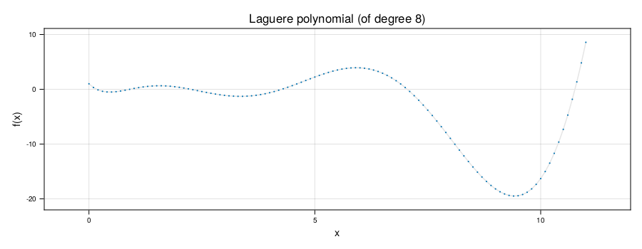

generalized_laguerreL(n::Integer, α, x::T; deriv=0, msg=true) where {T<:Real}

Generalized Laguerre polynomal of degree n for parameter α,

\[ L_{n}^{α}(x) = \frac{1}{n!}e^{x}x^{-α}\frac{d^{n}}{dx^{n}}(e^{-x}x^{n+α}) = \sum_{k=0}^{n}(-1)^{k}\binom{n+α}{n-k}\frac{x^{k}}{k!} = \sum_{k=0}^{n}c_k(n,α)x^{k}\]

where the $c_k(n,α)$ are the generalized Laguerre coefficients of generalized_laguerre_polynom.

Example:

julia> coords = generalized_laguerre_polynom(5, 3); println(coords)
Rational{Int64}[56//1, -70//1, 28//1, -14//3, 1//3, -1//120]

julia> polynomial(coords, 10.0)
-10.666666666667311

julia> generalized_laguerreL(5, 3, 10.0)
-10.666666666667311

laguerre_polynom(n::Integer [; msg=true])

The coefficients of laguerreL for degree n,

\[ v(n)=[c_0, c_1, \cdots\ c_n],\]

where

\[ c_k(n) = \frac{\Gamma(n+1)}{\Gamma(k+1)}\frac{(-1)^{k}}{(n-k)!}\frac{1}{k!}\]

with $k=0,1,⋯,n$.

• msg : integer-overflow protection (IOP) - warning on activation

Example:

julia> laguerre_polynom(7)
(1//1, -7//1, 21//2, -35//6, 35//24, -7//40, 7//720, -1//5040)

generalized_laguerre_polynom(n::Int [, α=0 [; msg=true]])

The coefficients of generalized_laguerreL for degree n and parameter α,

\[ v(n, α)=[c_0, c_1, \cdots\ c_n],\]

where

\[ c_k(n, α) = \frac{\Gamma(α+n+1)}{\Gamma(α+k+1)} \frac{(-1)^{k}}{(n-k)!}\frac{1}{k!}\]

with $k=0,1,⋯,n$.

• msg : integer-overflow protection (IOP) - warning on activation

Example:

julia> o =  generalized_laguerre_polynom(6,3); println(o)
Rational{Int64}[84//1, -126//1, 63//1, -14//1, 3//2, -3//40, 1//720]

julia> o =  generalized_laguerre_polynom(6,3.0); println(o)
[84.0, -126.0, 63.0, -14.0, 1.5, -0.075, 0.001388888888888889]

pascal_triangle(n::Integer [; arr=false [, msg=true]])

Row n of Pascal triangle, $r_n = [\binom{n}{1},\cdots\ \binom{n}{n}]$

• arr : output full Pascal triangle

• msg : integer-overflow protection (IOP) - warning on activation

(for n > 10000)

Examples:

julia> [pascal_triangle(n) for n=0:5]
6-element Vector{Vector{Int64}}:
 [1]
 [1, 1]
 [1, 2, 1]
 [1, 3, 3, 1]
 [1, 4, 6, 4, 1]
 [1, 5, 10, 10, 5, 1]

julia> pascal_triangle(5; arr=true)
5-element Vector{Vector{Int64}}:
 [1, 1]
 [1, 2, 1]
 [1, 3, 3, 1]
 [1, 4, 6, 4, 1]
 [1, 5, 10, 10, 5, 1]

pascal_next(row)

Next row of binomial coefficients of the Pascal triangle.

Example:

julia> pascal_next([1, 4, 6, 4, 1])
6-element Vector{Int64}:
  1
  5
 10
 10
  5
  1

permutations_unique_count(p::Vector{Vector{Integer}}, i::Int)

Number of unique permutations of the subarray $p[i]$.

Example:

p = [[1,2,3],[2,3,1,4,3]]
permutations_unique_count(p,2)
 60

pochhammer(x::T, p::Int) where T<:Real

Pochhammer symbol $(x)_{p}$ for non-negative integer p,

\[(x)_{p}=\begin{cases} 1 & p=0\\ x(x+1)(x+2)⋯(x+p-1) & p>0 \end{cases}\]

Note that $(x)_{p}=0$ for $x=0,-1,⋯\ -(p-1)$

Examples:

julia> x = [-4,-3,-2,-1, 0, 1, 2 , 3, 4];

julia> pochhammer.(x, 5) == [0, 0, 0, 0, 0, 120, 720, 2520, 6720]
true

julia> pochhammer.(x, 0) == [1, 1, 1, 1, 1, 1, 1, 1, 1]
true

julia> o = [pochhammer.([x for x=0:-1:-p],p) for p=0:5]
6-element Vector{Vector{Int64}}:
 [1]
 [0, -1]
 [0, 0, 2]
 [0, 0, 0, -6]        
 [0, 0, 0, 0, 24]     
 [0, 0, 0, 0, 0, -120]

julia>  o = [pochhammer.([x for x=0:p],p) for p=0:5]
6-element Vector{Vector{Int64}}:
 [1]
 [0, 1]
 [0, 2, 6]
 [0, 6, 24, 60]
 [0, 24, 120, 360, 840]
 [0, 120, 720, 2520, 6720, 15120]

julia> x = Rational{BigInt}(-1, 50);

julia> pochhammer(x, 20)
-21605762356630090481082546653745369902321614221999//9536743164062500000000000000000000

polynomial(coords, x::T [; deriv=0]) where {T<:Real}

Polynomial of degree $d$,

\[ P(x)=c_0 + c_1 x + ⋯ + c_d x^d,\]

where the coefficients coords = $(c_0,⋯\ c_d)$ define the vector representation of the polynomial in a vector space of dimension $d+1$.

Examples:

julia> coords = (1, 1, 1, 1, 1);
           
julia> P(x) = polynomial(coords,x);

julia> P(1)
5

julia> polynomial(coords, 1; deriv=1)     # P′(1)
10

julia> polynomial(coords, 2; deriv=2)     # P″(1)
20

julia> polynomial(coords,x; deriv=-1)   # primitive (zero integration constant)
137 // 60

polynom_power(coords, p)

The coords of a polynomial of degree $d$ raised to the power p, which define a polynomial in a vector space of dimension $p d + 1$.

Examples:

julia> coords = (1,1,1)    # coordinates of polynomial vector of degree d = 2
(1, 1, 1)

julia> coords = (1,1,1);

julia> polynom_power(coords, 3)
7-element Vector{Int64}:
 1
 3
 6
 7
 6
 3
 1

polynom_product(coords1, coords2)

The coefficients of the product of two polynomials, a = coords1 and b = coords2 of degree $m$ and $n$, which represents a polynomial in a vector space of dimension $d=m+n+1$,

\[ P(x)=a_0b_0 + (a_0b_1 + b_0a_1)x + ⋯ + a_n b_m x^{n+m}.\]

Examples:

julia> polynom_product((1, 1), (1, -1, 2))
4-element Vector{Int64}:
 1
 0
 1
 2

julia> polynom_product((1, 1), (1, -1.0, 2))
4-element Vector{Real}:
 1
 0.0
 1.0
 2  

polynom_product_expansion(coords1, coords2, p::Int)

The coefficients of the product of two polynomials, a = coords1 (of degree $n$) and b = coords2 (of degree $m$), truncated at the order p, which represents a polynomial in a vector space of dimension $d=p+1$

julia> a = (1,-1,1);

julia> b = (1,1,-1,1,1,1);

julia> o = polynom_product(a, b); println(o)
[1, 0, -1, 3, -1, 1, 0, 1]
 
julia> o = polynom_product_expansion(a, b, 4); println(o)
[1, 0, -1, 3, -1] 

istriangle(a::Real, b::Real, c::Real)

Triangle condition for a triangle of sides a, b and c.

Example:

julia> istriangle(3, 4, 5)
true

julia> istriangle(1//2, 1, 1.5)
true

triangle_coefficient(a::Real, b::Real, c::Real)

Triangle coefficient for a triangle of sides a, b and c,

\[ \Delta(abc)\equiv\frac{(a+b-c)!(b+c-a)!(c+a-b)!}{(a+b+c+1)!}\]

Triangle condition satisfied for $\Delta > 0$

Examples:

julia> triangle_coefficient(3, 4, 5)
1//180180

julia> triangle_coefficient(1//2, 1, 1.5)
1//12

threeJsymbol(j1::Real, m1::Real, j2::Real, m2::Real, j3::Real, m3::Real; msg=true)

Wigner 3j symbol. This is a vector coupling coefficient with optimized symmetry properties. The 3j symbols are zero unless $Δ(j_{1},j_{2},j_{3})>0$ (triangle inequality holds) and $m_{1}+m_{2}+m_{3}=0$. The implementation is based on the Racah formula:

\[\left(\begin{array}{ccc} j_{1} & j_{2} & j_{3}\\ m_{1} & m_{2} & m_{3} \end{array}\right)= (-1)^{j_{1}-j_{2}-m_{3}}\sqrt{\Delta(j_{1}j_{2}J)}\\\times \sqrt{\left(j_{1}+m_{1}\right)! \left(j_{1}-m_{1}\right)! \left(j_{2}+m_{2}\right)! \left(j_{2}-m_{2}\right)! \left(j_{3}+m_{3}\right)! \left(j_{3}-m_{3}\right)!} \\\times\sum_{t}\frac{(-)^{t}}{t!(j_{3}-j_{2}+t+m_{1})! (j_{3}-j_{1}+t-m_{2})! (j_{1}+j_{2}-j_{3}-t)!(j_{1}-t-m_{1})!(j_{2}-t+m_{2})!}\]

Example:

julia> o = threeJsymbol(3, 0, 4, -1, 5, 1); println(" = $o")
-√(361/30030) = -0.1096417439724123565166029917781360897459044055433631161836138910409772907333476

julia> threeJsymbol(3, 0, 4, -1, 5, 1; msg=false)
-0.1096417439724123565166029917781360897459044055433631161836138910409772907333476

julia> threeJsymbol(0, 0, 0, 0, 0, 0; msg=false)
1.0

CGC(j1::Real, m1::Real, j2::Real, m2::Real, J::Real, M::Real; msg=true)

Clebsch-Gordan coefficient (CGC). This is a vector-coupling coefficient in Dirac notation. The CGCs are zero unless $Δ(j_{1},j_{2},j_{3})>0$ (triangle inequality holds) and $M=m_{1}+m_{2}$. The relation to the Wigner 3j symbols is given by:

\[\langle j_{1}m_{1};j_{2}m_{2}|JM\rangle\equiv (-1)^{j_{1}-j_{2}+M}\sqrt{2J+1}\left(\begin{array}{ccc} j_{1} & j_{2} & J\\ m_{1} & m_{2} & -M \end{array}\right)\]

Example:

julia> j1=3; m1=0; j2=4; m2=-1; J=5; M=-1;

julia> o = CGC(j1, m1, j2, m2, J, M); println(" = $o")
-√(361/2730) = -0.36364052611670255269921486774521555203216489725107181148303161368088211274565

julia> o = CGC(j1, m1, j2, m2, J, M; msg=false); println(o)
-0.36364052611670255269921486774521555203216489725107181148303161368088211274565

julia> o = (-1)^(j1-j2+M) * sqrt(2J+1) * threeJsymbol(j1, m1, j2, m2, J, -M; msg=false); println(o)
-0.36364052611670255269921486774521555203216489725107181148303161368088211274565

julia> CGC(3, 0, 4, -1, 5, -1);
-√(361/2730)