PC Algorithm: Basic examples
A few example data sets can be useful to illustrate how to work with the PC algorithm and the different independence tests implemented in this package. The examples discussed here are based on the example models discussed in chapter 2 of Judea Pearl's book. The causal model we are going to study can be represented using the following DAG:
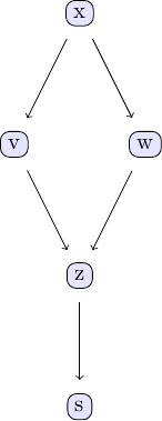
We can easily create some sample data that corresponds to the causal structure described by the DAG. For the sake of simplicity, let's create data from a simple linear model that follows the structure defined by the DAG shown above:
using CausalInference
using TikzGraphs
# If you have problems with TikzGraphs.jl,
# try alternatively plotting backend GraphRecipes.jl + Plots.jl
# and corresponding plotting function `plot_pc_graph_recipes`

# Generate some sample data to use with the PC algorithm

N = 1000 # number of data points

# define simple linear model with added noise
x = randn(N)
v = x + randn(N)*0.25
w = x + randn(N)*0.25
z = v + w + randn(N)*0.25
s = z + randn(N)*0.25

df = (x=x, v=v, w=w, z=z, s=s)
With this data ready, we can now see to what extent we can back out the underlying causal structure from the data using the PC algorithm. Under the hood, the PC algorithm uses repeated conditional independence tests to determine the causal relationships between different variables in a given data set. In order to run the PC algorithm on our test data set, we need to specify not only the data set we want to use, but also the conditional independence test alongside a p-value. For now, let's use a simple Gaussian conditional independence test with a p-value of 0.01.
est_g = pcalg(df, 0.01, gausscitest)In order to investigate the output of the PC algorithm, this package also provides a function to easily plot and visually analyse this output.
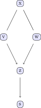
tp = plot_pc_graph_tikz(est_g, [String(k) for k in keys(df)])
The first thing that stands out in this plot is that only some edges have arrow marks, while others don't. For example, the edge going from v to z is pointing from v to z, indicating that that v influences z and not the other way around. On the other hand, the edge going from x to w has no arrows on either end, meaning that the direction of causal influence has not been identified and is in fact not identifiable based on the available data alone. Both causal directions, x influencing v and v influencing x, are compatible with the observed data. We can illustrate this directly by switching the direction of influence in the data generating process used above and running the PC algorithm for this new data set:
# Generate some additional sample data with different causal relationships

N = 1000 # number of data points

# define simple linear model with added noise
v = randn(N)
x = v + randn(N)*0.25
w = x + randn(N)*0.25
z = v + w + randn(N)*0.25
s = z + randn(N)*0.25

df = (x=x, v=v, w=w, z=z, s=s)

plot_pc_graph_tikz(pcalg(df, 0.01, gausscitest), [String(k) for k in keys(df)])
We can, however, conclude unequivocally from the available (observational) data alone that w and v are causal for z and z for s. At no point did we have to resort to things like direct interventions, experiments or A/B tests to arrive at these conclusions!