Low level interface

Since version 0.8.30 we strongly encourage the use of the ParticleSystem interface. Yet, the low level interface is still available. To use it, load the package as usual:

using CellListMap

Examples

The full code of the examples described here is available at the examples directory.

• Mean difference of coordinates
• Histogram of distances
• Gravitational potential
• Gravitational force
• Nearest neighbor
• Implementing Neighbor lists

Mean difference of coordinates

Computing the mean difference in x position between random particles. The closure is used to remove the indexes and the distance of the particles from the parameters of the input function, as they are not needed in this case.

using CellListMap

# System properties
N = 100_000
sides = [250,250,250]
cutoff = 10

# Particle positions
x = [ sides .* rand(3) for i in 1:N ]

# Initialize linked lists and box structures
box = Box(sides,cutoff)
cl = CellList(x,box)

# Function to be evaluated from positions 
f(x,y,sum_dx) = sum_dx + abs(x[1] - y[1])
normalization = N / (N*(N-1)/2) # (number of particles) / (number of pairs)

# Run calculation (0.0 is the initial value)
avg_dx = normalization * map_pairwise(
    (x,y,i,j,d2,sum_dx) -> f(x,y,sum_dx), 0.0, box, cl 
)

The example above can be run with CellListMap.Examples.average_displacement() and is available in the average_displacement.jl file.

Histogram of distances

Computing the histogram of the distances between particles (considering the same particles as in the above example). Again, we use a closure to remove the positions and indexes of the particles from the function arguments, because they are not needed. The distance, on the other side, is needed in this example:

# Function that accumulates the histogram of distances
function build_histogram!(d2,hist)
    d = sqrt(d2)
    ibin = floor(Int,d) + 1
    hist[ibin] += 1
    return hist
end;

# Initialize (and preallocate) the histogram
hist = zeros(Int,10);

# Run calculation
map_pairwise!(
    (x,y,i,j,d2,hist) -> build_histogram!(d2,hist),
    hist,box,cl
)

Note that, since hist is mutable, there is no need to assign the output of map_pairwise! to it.

The example above can be run with CellListMap.Examples.distance_histogram() and is available in the distance_histogram.jl file.

Gravitational potential

In this test we compute the "gravitational potential", assigning to each particle a different mass. In this case, the closure is used to pass the masses to the function that computes the potential.

# masses
const mass = rand(N)

# Function to be evaluated for each pair 
function potential(i,j,d2,mass,u)
    d = sqrt(d2)
    u = u - 9.8*mass[i]*mass[j]/d
    return u
end

# Run pairwise computation
u = map_pairwise((x,y,i,j,d2,u) -> potential(i,j,d2,mass,u),0.0,box,cl)

The example above can be run with CellListMap.Examples.gravitational_potential() and is available in the gravitational_potential.jl file.

Gravitational force

In the following example, we update a force vector of for all particles.

# masses
const mass = rand(N)

# Function to be evaluated for each pair: update force vector
function calc_forces!(x,y,i,j,d2,mass,forces)
    G = 9.8*mass[i]*mass[j]/d2
    d = sqrt(d2)
    df = (G/d)*(x - y)
    forces[i] = forces[i] - df
    forces[j] = forces[j] + df
    return forces
end

# Initialize and preallocate forces
forces = [ zeros(SVector{3,Float64}) for i in 1:N ]

# Run pairwise computation
map_pairwise!(
    (x,y,i,j,d2,forces) -> calc_forces!(x,y,i,j,d2,mass,forces),
    forces,box,cl
)

The example above can be run with CellListMap.Examples.gravitational_force() and is available in the gravitational_force.jl file.

Nearest neighbor

Here we compute the indexes of the particles that satisfy the minimum distance between two sets of points, using the linked lists. The distance and the indexes are stored in a tuple, and a reducing method has to be defined for that tuple to run the calculation. The function does not need the coordinates of the points, only their distance and indexes.

# Number of particles, sides and cutoff
N1=1_500
N2=1_500_000
sides = [250,250,250]
cutoff = 10.
box = Box(sides,cutoff)

# Particle positions
x = [ SVector{3,Float64}(sides .* rand(3)) for i in 1:N1 ]
y = [ SVector{3,Float64}(sides .* rand(3)) for i in 1:N2 ]

# Initialize auxiliary linked lists
cl = CellList(x,y,box)

# Function that keeps the minimum distance
f(i,j,d2,mind) = d2 < mind[3] ? (i,j,d2) : mind

# We have to define our own reduce function here
function reduce_mind(output,output_threaded)
    mind = output_threaded[1]
    for i in 2:length(output_threaded)
        if output_threaded[i][3] < mind[3]
            mind = output_threaded[i]
        end
    end
    return mind
end

# Initial value
mind = ( 0, 0, +Inf )

# Run pairwise computation
mind = map_pairwise( 
    (x,y,i,j,d2,mind) -> f(i,j,d2,mind),
    mind,box,cl;reduce=reduce_mind
)

The example above can be run with CellListMap.Examples.nearest_neighbor() and is available in the nearest_neighbor.jl file.

The example CellListMap.Examples.nearest_neighbor_nopbc() of nearest_neighbor_nopbc.jl describes a similar problem but without periodic boundary conditions. Depending on the distribution of points and size it is a faster method than usual ball-tree methods.

Implementing Neighbor lists

The implementation of the CellLIstMap.neighborlist (see Neighbor lists) is as follows: The empty pairs output array will be split in one vector for each thread, and reduced with a custom reduction function.

# Function to be evaluated for each pair: push pair
function push_pair!(i,j,d2,pairs)
    d = sqrt(d2)
    push!(pairs,(i,j,d))
    return pairs
end

# Reduction function
function reduce_pairs(pairs,pairs_threaded)
    for i in eachindex(pairs_threaded)
        append!(pairs,pairs_threaded[i])
    end
    return pairs
end

# Initialize output
pairs = Tuple{Int,Int,Float64}[]

# Run pairwise computation
map_pairwise!(
    (x,y,i,j,d2,pairs) -> push_pair!(i,j,d2,pairs),
    pairs,box,cl,
    reduce=reduce_pairs
)

The full example can be run with CellListMap.Examples.neighborlist(), available in the file neighborlist.jl.

Periodic boundary conditions

• Orthorhombic periodic boundary conditions
• Triclinic periodic boundary conditions
• Without periodic boundary conditions

Orthorhombic periodic boundary conditions

Orthorhombic periodic boundary conditions allow some special methods that are faster than those for general cells. To initialize an Orthorhombic cell, just provide the length of the cell on each side, and the cutoff. For example:

julia> box = Box([100,70,130],12)
Box{OrthorhombicCell, 3, Float64, 9}
  unit cell matrix: [100.0 0.0 0.0; 0.0 70.0 0.0; 0.0 0.0 130.0]
  cutoff: 12.0
  number of computing cells on each dimension: [10, 7, 12]
  computing cell sizes: [12.5, 14.0, 13.0] (lcell: 1)
  Total number of cells: 840

Triclinic periodic boundary conditions

Triclinic periodic boundary conditions of any kind can be used. However, the input has some limitations for the moment. The lattice vectors must have strictly positive coordinates, and the smallest distance within the cell cannot be smaller than twice the size of the cutoff. An error will be produced if the cell does not satisfy these conditions.

Let us illustrate building a two-dimensional cell, for easier visualization. A matrix of column-wise lattice vectors is provided in the construction of the box, and that is all.

Here, the lattice vectors are [1,0] and [0.5,1] (and we illustrate with cutoff=0.1):

julia> box = Box([ 1.0  0.5
                   0.0  1.0 ], 0.1);

julia> x = 10*rand(SVector{2,Float64},1000);

We have created random coordinates for 1000 particles, that are not necessarily wrapped according to the periodic boundary conditions. We can see the coordinates in the minimum image cell with:

julia> using Plots

julia> CellListMap.draw_computing_cell(x,box)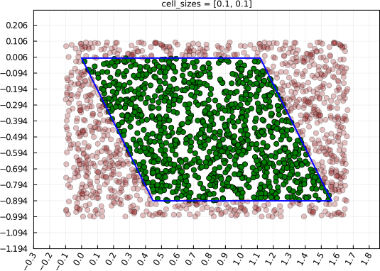

The construction of the cell list is, as always, done with:

julia> cl = CellList(x,box)
CellList{2, Float64}
  109 cells with real particles.
  2041 particles in computing box, including images.

Upon construction of the cell lists, the cell is rotated such that the longest axis becomes oriented along the x-axis, and the particles are replicated to fill a rectangular box (or orthorhombic box, in three-dimensions), with boundaries that exceed the actual system size. This improves the performance of the pairwise computations by avoiding the necessity of wrapping coordinates on the main loop (these is an implementation detail only).

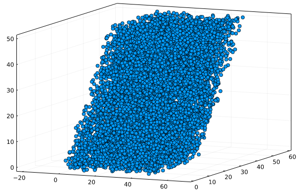
In summary, to use arbitrary periodic boundary conditions, just initialize the box with the matrix of lattice vectors. In three dimensions, for example, one could use:

julia> unitcell = [ 50.  0. 00. 
                     0. 30. 30.          
                     0. 00. 50. ]

julia> box = Box(unitcell,  2.)

julia> x = 100*rand(SVector{3,Float64},10000);

julia> p = [ CellListMap.wrap_to_first(x,unitcell) for x in x ];

julia> using Plots

julia> scatter(Tuple.(p),aspect_ratio=1,framestyle=:box,label=:none)

to work with an arbitrary 3D lattice, Which in this case looks like:

Without periodic boundary conditions

To avoid the use of periodic boundary conditions it is enough to define an Orthorhombic box with lengths in each direction that are larger than the limits of the coordinates of the particles plus the cutoff. This can be done automatically with the limits function. The box must be constructed with:

julia> x = [ [100,100,100] .* rand(3) for i in 1:100_000 ];

julia> box = Box(limits(x),12)
Box{NonPeriodicCell, 3}
  unit cell matrix = [ 112.0, 0.0, 0.0; 0.0, 112.0, 0.0; 0.0, 0.0, 112.0 ]
  cutoff = 12.0
  number of computing cells on each dimension = [11, 11, 11]
  computing cell sizes = [12.44, 12.44, 12.44] (lcell: 1)
  Total number of cells = 1331

or, for computing the interaction between two disjoint sets of particles, call the limits function with two arguments:

julia> x = [ [100,100,100] .* rand(3) for i in 1:100_000 ];

julia> y = [ [120,180,100] .* rand(3) for i in 1:100_000 ];

julia> box = Box(limits(x,y),12)
Box{NonPeriodicCell, 3}
  unit cell matrix = [ 132.0, 0.0, 0.0; 0.0, 192.0, 0.0; 0.0, 0.0, 112.0 ]
  cutoff = 12.0
  number of computing cells on each dimension = [12, 17, 11]
  computing cell sizes = [13.2, 12.8, 12.44] (lcell: 1)
  Total number of cells = 2244

Note that the unit cell length is, on each direction, the maximum coordinates of all particles plus the cutoff. This will avoid the computation of pairs of periodic images. The algorithms used for computing interactions in Orthorhombic cells will then be used.

Parallelization splitting and reduction

• How output is updated thread-safely
• Custom reduction functions
• Number of batches

The parallel execution requires the splitting of the computation among tasks.

How output is updated thread-safely

To allow general output types, the approach of CellListMap is to copy the output variable the number of times necessary for each parallel task to update an independent output variables, which are reduced at the end. This, of course, requires some additional memory, particularly if the output being updated is formed by arrays. These copies can be preallocated, and custom reduction functions can be defined.

To control these steps, set manually the output_threaded and reduce optional input parameters of the map_pairwise! function.

By default, we define:

output_threaded = [ deepcopy(output) for i in 1:nbatches(cl) ]

where nbatches(cl) is the number of batches into which the computation will be divided. The number of batches is not necessarily equal to the number of threads available (an heuristic is used to optimize performance, as a function of the workload per batch), but can be manually set, as described in the Number of batches section below.

The default reduction function just assumes the additivity of the results obtained by each batch:

reduce(output::Number,output_threaded) = sum(output_threaded)
function reduce(output::Vector,output_threaded) 
    @. output = output_threaded[1]
    for i in 2:length(output_threaded)
         @. output += output_threaded[i] 
    end
    return output
end

Custom reduction functions

In some cases, as in the Nearest neighbor example, the output is a tuple and reduction consists in keeping the output from each thread having the minimum value for the distance. Thus, the reduction operation is not a simple sum over the elements of each threaded output. We can, therefore, overwrite the default reduction method, by passing the reduction function as the reduce parameter of map_pairwise!:

mind = map_pairwise!( 
    (x,y,i,j,d2,mind) -> f(i,j,d2,mind), mind,box,cl;
    reduce=reduce_mind
)

where here the reduce function is set to be the custom function that keeps the tuple associated to the minimum distance obtained between threads:

function reduce_mind(output,output_threaded)
    mind = output_threaded[1]
    for i in 2:length(output_threaded)
        if output_threaded[i][3] < mind[3]
            mind = output_threaded[i]
        end
    end
    return mind
end

This function must return the updated output variable, being it mutable or not, to be compatible with the interface.

Using the length of the output_threaded vector as the measure of how many copies of the array is available is convenient because it will be insensitive in changes in the number of batches that may be set.

Number of batches

Every calculation with cell lists has two steps: the construction of the lists, and the mapping of the computation among the pairs of particles that satisfy the cutoff criterion.

The construction of the cell list is harder to parallelize, because assigning each particle to a cell is fast, such that the cost of merging a set of lists generated in parallel can be as costly as building the lists themselves. Therefore, it is frequent that it is not worthwhile (actually it is detrimental for performance) to split the construction of the cell lists in too many threads. This is particularly relevant for smaller systems, for which the cost of constructing the lists can be comparable to the cost of actually computing the mapped function.

At the same time, the homogeneity of the computation of the mapped function may be fast or not, homogeneous or not. These characteristics affect the optimal workload splitting strategy. For very large systems, or systems for which the function to be computed is not homogeneous in time, it may be interesting to split the workload in many tasks as possible, such that slow tasks do not dominate the final computational time.

Both the above considerations can be used to tunning the nbatches parameter of the cell list. This parameter is initialized from a tuple of integers, defining the number of batches that will be used for constructing the cell lists and for the mapping of the computations.

By default, the number of batches for the computation of the cell lists is smaller than nthreads() if the number of particles per cell is small. The default value by the internal function CellListMap._nbatches_build_cell_lists(cl::CellList).

The values assumed for each number of batches can bee seen by printing the nbatches parameter of the cell lists:

julia> Threads.nthreads()
64

julia> x, box = CellListMap.xatomic(10^4) # random set with atomic density of water

julia> cl = CellList(x,box);

julia> cl.nbatches
NumberOfBatches
  Number of batches for cell list construction: 8 
  Number of batches for function mapping: 32 

The construction of the cell lists is performed by creating copies of the data, and currently does not scale very well. Thus, no more than 8 batches are used by default, to avoid delays associated to data copying and garbage collection. The number of batches of the mapping function uses an heuristic which currently limits somewhat the number of batches for small systems, when the overhead of spawning tasks is greater than the computation. Using more batches than threads for the function mapping is effective most times in avoiding uneven workload, but it may be a problem if the output to be reduced is too large, as the threaded version of the output contains nbatches copies of the output.

Using less batches than the number of threads also allows the efficient use of nested multi-threading, as the computations will only use the number of threads required, leaving the other threads available for other tasks.

The number of batches is set on the construction of the cell list, using the nbatches keyword parameter. For example:

julia> cl = CellList(x,box,nbatches=(1,4))
CellList{3, Float64}
  1000000 real particles.
  1000 cells with real particles.
  1727449 particles in computing box, including images.

julia> cl.nbatches
NumberOfBatches
  Number of batches for cell list construction: 1
  Number of batches for function mapping: 4

fine tunning of the performance for a specific problem can be obtained by adjusting this parameter.

If the number of batches is set as zero for any of the two options, the default value is retained. For example:

julia> cl = CellList(x,box,nbatches=(0,4));

julia> cl.nbatches
NumberOfBatches
  Number of batches for cell list construction: 8 
  Number of batches for function mapping: 4

julia> cl = CellList(x,box,nbatches=(4,0));

julia> cl.nbatches
NumberOfBatches
  Number of batches for cell list construction: 4
  Number of batches for function mapping: 64

The number of batches can also be retrieved from the cell list using the nbatches function:

julia> cl = CellList(x,box,nbatches=(2,4));

julia> cl.nbatches
NumberOfBatches
  Number of batches for cell list construction: 2
  Number of batches for function mapping: 4

julia> nbatches(cl) # returns cl.nbatches.map_computation
4

julia> nbatches(cl,:map) # returns cl.nbatches.map_computation
4

julia> nbatches(cl,:build) # returns cl.nbatches.build_cell_lists
2

The call nbatches(cl) is important for defining the number of copies of preallocated threaded output variables, as explained in the previous section.

Performance tunning and additional options

• Preallocating the cell lists and cell list auxiliary arrays
• Preallocating threaded output auxiliary arrays
• Optimizing the cell grid

Preallocating the cell lists and cell list auxiliary arrays

The arrays containing the cell lists can be initialized only once, and then updated. This is useful for iterative runs. Note that, since the list size depends on the box size and cutoff, if the box properties changes some arrays might be increased (never shrink) on this update.

# Initialize cell lists with initial coordinates
cl = CellList(x,box)
# Allocate auxiliary arrays for threaded cell list construction
aux = CellListMap.AuxThreaded(cl)
for i in 1:nsteps
    x = ... # new coordinates
    box = Box(sides,cutoff) # perhaps the box has changed
    UpdateCellList!(x,box,cl,aux) # modifies cl
    map_pairwise!(...)
end

The procedure is identical if using two sets of coordinates, in which case, one would do:

cl = CellList(x,y,box)
aux = CellListMap.AuxThreaded(cl)
for i in 1:nsteps
    x = ... # new coordinates
    box = Box(sides,cutoff) # perhaps the box has changed
    UpdateCellList!(x,y,box,cl,aux) # modifies cl
    map_pairwise(...)
end

By passing the aux auxiliary structure, the UpdateCellList! functions will only allocate some minor variables associated to the launching of multiple threads and, possibly, to the expansion of the cell lists if the box or the number of particles became greater.

Preallocating threaded output auxiliary arrays

On parallel runs, note that output_threaded is, by default, initialized on the call to map_pairwise!. Thus, if the calculation must be run multiple times (for example, for several steps of a trajectory), it is probably a good idea to preallocate the threaded output, particularly if it is a large array. For example, the arrays of forces should be created only once, and reset to zero after each use:

forces = zeros(SVector{3,Float64},N)
forces_threaded = [ deepcopy(forces) for i in 1:nbatches(cl) ]
for i in 1:nsteps
    map_pairwise!(f, forces, box, cl, output_threaded=forces_threaded)
    # work with the final forces vector
    ...
    # Reset forces_threaded
    for i in 1:nbatches(cl)
        @. forces_threaded[i] = zero(SVector{3,Float64}) 
    end
end

In this case, the forces vector will be updated by the default reduction method. nbatches(cl) is the number of batches of the parallel calculation, which is defined on the construction of the cell list (see the Parallelization section).

Optimizing the cell grid

The partition of the space into cells is dependent on a parameter lcell which can be passed to Box. For example:

box = Box(x,box,lcell=2)
cl = CellList(x,box)
map_pairwise!(...)

This parameter determines how fine is the mesh of cells. There is a trade-off between the number of cells and the number of particles per cell. For low-density systems, greater meshes are better, because each cell will have only a few particles and the computations loop over a smaller number of cells. For dense systems, it is better to run over more cells with less particles per cell. It is a good idea to test different values of lcell to check which is the optimal choice for your system. Usually the best value is lcell=1, because in CellListMap implements a method to avoid spurious computations of distances on top of the cell lists, but for very dense systems, or for very large cutoffs (meaning, for situations in which the number of particles per cell may be very large), a greater lcell may provide a better performance. It is unlikely that lcell > 3 is useful in any practical situation. For molecular systems with normal densities lcell=1 is likely the optimal choice. The performance can be tested using the progress meter, as explained below.

As a rough guide, lcell > 1 is only worthwhile if the number of particles per cell is greater than ~200-400.

Output progress

For long-running computations, the user might want to see the progress. A progress meter can be turned on with the show_progress option. For example:

map_pairwise!(f,output,box,cl,show_progress=true)

will print something like:

Progress:  43%|█████████████████                    | ETA: 0:18:25

Thus, besides being useful for following the progress of a long run, it is useful to test different values of lcell to tune the performance of the code, by looking at the estimated time to finish (ETA) and killing the execution after a sample run. The default and recommended option for production runs is to use show_progress=false, because tracking the progress introduces a small overhead into the computation.

Some benchmarks

Computing a histogram of pairwise velocities

The goal here is to provide a good implementation of cell lists. We compare it with the implementation of the nice cython/python halotools package, in the computation of an histogram of mean pairwise velocities.

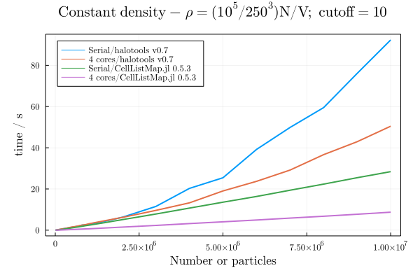
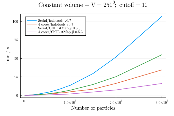
The full test is available at this repository. And we kindly thank Carolina Cuesta for providing the example. These benchmarks were run on an Intel i7 8th gen laptop, with 4 cores (8 threads).

Additional options

Input coordinates as matrices

For compatibility with other software, the input coordinates can be provided as matrices. The matrices must have dimensions (2,N) or (3,N), where N is the number of particles (because Julia is column-major, thus this has the same memory layout of an array of length N of static vectors).

For example:

julia> x = rand(3,100);

julia> box = Box([1,1,1],0.1);

julia> cl = CellList(x,box)
CellList{3, Float64}
  100 real particles.
  99 cells with real particles.
  162 particles in computing box, including images.

julia> map_pairwise!((x,y,i,j,d2,n) -> n += 1, 0, box, cl) # count neighbors
23

Docstrings

Box(unitcell::Limits, cutoff; lcell::Int=1)

julia> using CellListMap, PDBTools

julia> x = coor(readPDB(CellListMap.argon_pdb_file));

julia> box = Box(limits(x), 10.0)
Box{NonPeriodicCell, 3}
  unit cell matrix = [ 39.83 0.0 0.0; 0.0 39.96 0.0; 0.0 0.0 39.99 ]
  cutoff = 10.0
  number of computing cells on each dimension = [6, 6, 6]
  computing cell sizes = [13.28, 13.32, 13.33] (lcell: 1)
  Total number of cells = 216

julia> y = 1.2 .* x;

julia> box = Box(limits(x,y),10)
Box{NonPeriodicCell, 3}
  unit cell matrix = [ 43.6 0.0 0.0; 0.0 43.76 0.0; 0.0 0.0 43.79 ]
  cutoff = 10.0
  number of computing cells on each dimension = [7, 7, 7]
  computing cell sizes = [10.9, 10.94, 10.95] (lcell: 1)
  Total number of cells = 343

Box(unit_cell_matrix::AbstractMatrix, cutoff, lcell::Int=1, UnitCellType=TriclinicCell)

julia> using CellListMap 

julia> unit_cell = [ 100   50    0 
                       0  120    0
                       0    0  130 ];

julia> box = Box(unit_cell, 10.0)
Box{TriclinicCell, 3}
  unit cell matrix = [ 100.0 0.0 0.0; 50.0 120.0 0.0; 0.0 0.0 130.0 ]
  cutoff = 10.0
  number of computing cells on each dimension = [20, 13, 16]
  computing cell sizes = [10.0, 10.0, 10.0] (lcell: 1)
  Total number of cells = 4160

julia> using CellListMap

julia> unit_cell = [ 100 0 0; 0 120 0; 0 0 150 ]; # cell is orthorhombic

julia> box = Box(unit_cell, 10.0, UnitCellType=OrthorhombicCell) # forcing OrthorhombicCell
Box{OrthorhombicCell, 3}
  unit cell matrix = [ 100.0 0.0 0.0; 0.0 120.0 0.0; 0.0 0.0 150.0 ]
  cutoff = 10.0
  number of computing cells on each dimension = [13, 15, 18]
  computing cell sizes = [10.0, 10.0, 10.0] (lcell: 1)
  Total number of cells = 3510

Box(sides::AbstractVector, cutoff, lcell::Int=1, UnitCellType=OrthorhombicCell)

julia> using CellListMap

julia> box = Box([120,150,100],10)
Box{OrthorhombicCell, 3}
  unit cell matrix = [ 120.0 0.0 0.0; 0.0 150.0 0.0; 0.0 0.0 100.0 ]
  cutoff = 10.0
  number of computing cells on each dimension = [15, 18, 13]
  computing cell sizes = [10.0, 10.0, 10.0] (lcell: 1)
  Total number of cells = 3510

unitcelltype(::Box{T}) where T = T

julia> using CellListMap

julia> box = Box([1,1,1], 0.1);

julia> unitcelltype(box)
OrthorhombicCell

julia> box = Box([1 0 0; 0 1 0; 0 0 1], 0.1);

julia> unitcelltype(box)
TriclinicCell

map_pairwise(args...;kargs...) = map_pairwise!(args...;kargs...)

map_pairwise!(
    f::Function,
    output,
    box::Box,
    cl::CellList
    ;parallel::Bool=true,
    show_progress::Bool=false
)

f(x,y,i,j,d2,output)

julia> n = 100_000;

julia> box = Box([250,250,250],10);

julia> x = [ SVector{3,Float64}(sides .* rand(3)) for i in 1:n ];

julia> cl = CellList(x,box);

julia> f(x,y,sum_dx) = sum_dx + abs(x[1] - y[1])

julia> normalization = N / (N*(N-1)/2) # (number of particles) / (number of pairs)

julia> avg_dx = normalization * map_parwise!((x,y,i,j,d2,sum_dx) -> f(x,y,sum_dx), 0.0, box, cl)

map_pairwise!(f::Function,output,box::Box,cl::CellListPair)

AuxThreaded(cl::CellListPair{N,T}) where {N,T}

julia> box = Box([250,250,250],10);

julia> x = [ 250*rand(3) for i in 1:50_000 ];

julia> y = [ 250*rand(3) for i in 1:10_000 ];

julia> cl = CellList(x,y,box);

julia> aux = CellListMap.AuxThreaded(cl)
CellListMap.AuxThreaded{3, Float64}
 Auxiliary arrays for nthreads = 8

julia> UpdateCellList!(x,box,cl,aux)
CellList{3, Float64}
  100000 real particles.
  31190 cells with real particles.
  1134378 particles in computing box, including images.

AuxThreaded(cl::CellList{N,T}) where {N,T}

julia> box = Box([250,250,250],10);

julia> x = [ 250*rand(3) for _ in 1:100_000 ];

julia> cl = CellList(x,box);

julia> aux = CellListMap.AuxThreaded(cl)
CellListMap.AuxThreaded{3, Float64}
 Auxiliary arrays for nthreads = 8

julia> UpdateCellList!(x,box,cl,aux)
CellList{3, Float64}
  100000 real particles.
  31190 cells with real particles.
  1134378 particles in computing box, including images.

CellList(
    x::AbstractVector{<:AbstractVector},
    y::AbstractVector{<:AbstractVector},
    box::Box{UnitCellType,N,T};
    parallel::Bool=true,
    nbatches::Tuple{Int,Int}=(0,0),
    autoswap::Bool=true
) where {UnitCellType,N,T}

julia> box = Box([250,250,250],10);

julia> x = [ 250*rand(SVector{3,Float64}) for i in 1:1000 ];

julia> y = [ 250*rand(SVector{3,Float64}) for i in 1:10000 ];

julia> cl = CellList(x,y,box)
CellListMap.CellListPair{Vector{SVector{3, Float64}}, 3, Float64}
   10000 particles in the reference vector.
   961 cells with real particles of target vector.

julia> cl = CellList(x,y,box,autoswap=false)
CellListMap.CellListPair{Vector{SVector{3, Float64}}, 3, Float64}
   1000 particles in the reference vector.
   7389 cells with real particles of target vector.

CellList(
    x::AbstractVector{AbstractVector},
    box::Box{UnitCellType,N,T};
    parallel::Bool=true,
    nbatches::Tuple{Int,Int}=(0,0)
) where {UnitCellType,N,T}

julia> box = Box([250,250,250],10);

julia> x = [ 250*rand(SVector{3,Float64}) for i in 1:100000 ];

julia> cl = CellList(x,box)
CellList{3, Float64}
  100000 real particles.
  15600 cells with real particles.
  126276 particles in computing box, including images.

UpdateCellList!(
    x::AbstractVector{<:AbstractVector},
    y::AbstractVector{<:AbstractVector},
    box::Box,
    cl:CellListPair,
    parallel=true
)

julia> box = Box([250,250,250],10);

julia> x = [ 250*rand(SVector{3,Float64}) for i in 1:1000 ];

julia> y = [ 250*rand(SVector{3,Float64}) for i in 1:10000 ];

julia> cl = CellList(x,y,box);

julia> UpdateCellList!(x,y,box,cl); # update lists

UpdateCellList!(
    x::AbstractVector{<:AbstractVector},
    box::Box,
    cl:CellList,
    parallel=true
)

julia> box = Box([250,250,250],10);

julia> x = [ 250*rand(SVector{3,Float64}) for i in 1:1000 ];

julia> cl = CellList(x,box);

julia> box = Box([260,260,260],10);

julia> x = [ 260*rand(SVector{3,Float64}) for i in 1:1000 ];

julia> UpdateCellList!(x,box,cl); # update lists

UpdateCellList!(
    x::AbstractVector{<:AbstractVector},
    y::AbstractVector{<:AbstractVector},
    box::Box,
    cl_pair::CellListPair,
    aux::Union{Nothing,AuxThreaded};
    parallel::Bool=true
)

julia> box = Box([250,250,250],10);

julia> x = [ 250*rand(3) for i in 1:50_000 ];

julia> y = [ 250*rand(3) for i in 1:10_000 ];

julia> cl = CellList(x,y,box)
CellListMap.CellListPair{Vector{SVector{3, Float64}}, 3, Float64}
   50000 particles in the reference vector.
   7381 cells with real particles of target vector.

julia> aux = CellListMap.AuxThreaded(cl)
CellListMap.AuxThreaded{3, Float64}
 Auxiliary arrays for nthreads = 8

julia> x = [ 250*rand(3) for i in 1:50_000 ];

julia> y = [ 250*rand(3) for i in 1:10_000 ];

julia> UpdateCellList!(x,y,box,cl,aux)
CellList{3, Float64}
  10000 real particles.
  7358 cells with real particles.
  12591 particles in computing box, including images.

julia> using BenchmarkTools

julia> @btime UpdateCellList!($x,$y,$box,$cl,$aux)
  715.661 μs (41 allocations: 3.88 KiB)
CellListMap.CellListPair{Vector{SVector{3, Float64}}, 3, Float64}
   50000 particles in the reference vector.
   7414 cells with real particles of target vector.
   
julia> @btime UpdateCellList!($x,$y,$box,$cl,$aux,parallel=false)
   13.042 ms (0 allocations: 0 bytes)
 CellListMap.CellListPair{Vector{SVector{3, Float64}}, 3, Float64}
    50000 particles in the reference vector.
    15031 cells with real particles of target vector.
 

UpdateCellList!(
    x::AbstractVector{<:AbstractVector},
    box::Box,
    cl::CellList{N,T},
    aux::Union{Nothing,AuxThreaded{N,T}};
    parallel::Bool=true
) where {N,T}

julia> box = Box([250,250,250],10);

julia> x = [ 250*rand(SVector{3,Float64}) for i in 1:100000 ];

julia> cl = CellList(x,box);

julia> aux = CellListMap.AuxThreaded(cl)
CellListMap.AuxThreaded{3, Float64}
 Auxiliary arrays for nthreads = 8

julia> x = [ 250*rand(SVector{3,Float64}) for i in 1:100000 ];

julia> UpdateCellList!(x,box,cl,aux)
CellList{3, Float64}
  100000 real particles.
  15599 cells with real particles.
  125699 particles in computing box, including images.

julia> using BenchmarkTools

julia> @btime UpdateCellList!($x,$box,$cl,$aux)
  16.384 ms (41 allocations: 3.88 KiB)
CellList{3, Float64}
  100000 real particles.
  15599 cells with real particles.
  125699 particles in computing box, including images.

julia> @btime UpdateCellList!($x,$box,$cl,$aux,parallel=false)
  20.882 ms (0 allocations: 0 bytes)
CellList{3, Float64}
  100000 real particles.
  15603 cells with real particles.
  125896 particles in computing box, including images.

nbatches(cl)

julia> x = rand(3,1000); box = Box([1,1,1],0.1);

julia> cl = CellList(x,box,nbatches=(2,16));

julia> nbatches(cl)
16

julia> nbatches(cl,:map)
16

julia> nbatches(cl,:build)
2

limits(x,y)

limits(x)