Detrended Cross-Correlation Analysis
A module to perform DCCA coefficients analysis. The coefficient describes the correlation strengh between two time series depending on time scales. it lies in [-1, 1], 1 being perfect correlations, and -1 perfect anticorrelations.
The package provides also functions returning a 95% confidence interval for the null-hypothesis (= "no-correlations").
| Travis |
|---|
 |
The implementation is based on Zebende G, Da Silva M MacHado, Filho A. DCCA cross-correlation coefficient differentiation: Theoretical and practical approaches Physica A: Statistical Mechanics and its Applications (2013) and was tested by reproducing the results of DCCA and DMCA correlations of cryptocurrency markets from Paulo Ferreira, Ladislav Kristoufk and Eder Johnson de Area LeãoPereira.
Perform a DCCA coefficient computation :
Call the rhoDCCA function like :
pts, rho = rhoDCCA(timeSeries1, timeSeries2)
The function rhoDCCA(timeSeries1, timeSeries2; box_start = 3, box_stop = div(length(data1),10), nb_pts = 30) has the following input arguments :
timeSeries1, timeSeries2: the time series to analyse (have to be array of Float64), having the same length.box_start = 3, box_stop: the starting and ending point of the analysis. defaults to 3 (the minimal possible time-scale) and 1/10th of the data length (passed this size the variance gets big).nb_pt: the number of points you want to evalute the analysis onto. mostly relevant for plotting
Returns :
pts: the list of points where the analysis was carried outrho: the value of the DCCA coefficient at each of these points
Get the 95% confidence interval
As a rule of thumb : values of rho in [-0.1,0.1] usually aren't significant.
The confidence intervals provided by this package correspond to the null-hypothesis i.e no correlations. If rho gets outside of this interval it can be considered significant.
To get a fast estimation of the confidence interval, call the empirical_CI function like : pts, ci = empirical_CI(dataLength).
For a more accurate estimation, you can call bootstrap_CI : pts, ci = bootstrap_CI(timeSeries1, timeSeries2; iterations = 200). This operation is much more demanding and can take up to several minutes. The iterations additional argument controls the number of repetitions for the bootstrap procedure, the higher the value, the smoother and cleaner the estimation will be, but it will also take longer.
Example of simple analysis :
calling the DCCA function with random white noise
julia> x1 = rand(2000); x2 = rand(2000)
x,y = rhoDCCA(x1,x2)
pts, ci = empirical_CI(length(x1))
Gave the following plot :
a = scatter(x,y, markersize = 7, xscale = :log, title = "Example of DCCA analysis : \n Correlations between two white noise time series", label = "rho coefficients", xlabel = "window sizes", ylabel = "Correlation strengh")
plot!(a,pts,ci, color = "red", linestyle = :dot, label = "limits of null-hypothesis")
plot!(a,pts,-ci, color = "red", linestyle = :dot, label = "")
display(a)
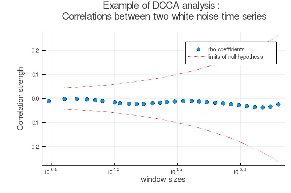 As noted previously, the value here lies in [-0.1,0.1] although we took here 2 series of white uncorrelated noise.
Installation :
julia> Using Pkg
Pkg.clone("https://github.com/johncwok/DCCA.jl.git")
TO DO :
- More user-friendly design ?
- Better figure for the readme file.