Nearest neighbor estimators
Kraskov
Entropies.Kraskov — Typek-th nearest neighbour(kNN) based
Kraskov(; k::Int = 1, w::Int = 0) <: EntropyEstimatorEntropy estimator based on k-th nearest neighbor searches[Kraskov2004]. w is the Theiler window.
This estimator is only available for entropy estimation. Probabilities cannot be obtained directly.
Kozachenko-Leonenko
Entropies.KozachenkoLeonenko — TypeKozachenkoLeonenko(; k::Int = 1, w::Int = 0) <: EntropyEstimatorEntropy estimator based on nearest neighbors. This implementation is based on Kozachenko & Leonenko (1987)[KozachenkoLeonenko1987], as described in Charzyńska and Gambin (2016)[Charzyńska2016].
w is the Theiler window (defaults to 0, meaning that only the point itself is excluded when searching for neighbours).
This estimator is only available for entropy estimation. Probabilities cannot be obtained directly.
Example
This example reproduces Figure in Charzyńska & Gambin (2016)[Charzyńska2016]. Both estimators nicely converge to the true entropy with increasing time series length. For a uniform 1D distribution $U(0, 1)$, the true entropy is 0 (red line).
using Entropies, DelayEmbeddings, StatsBase
import Distributions: Uniform, Normal

Ns = [100:100:500; 1000:1000:10000]
Ekl = Vector{Vector{Float64}}(undef, 0)
Ekr = Vector{Vector{Float64}}(undef, 0)

est_nn = KozachenkoLeonenko(w = 0)
# with k = 1, Kraskov is virtually identical to KozachenkoLeonenko, so pick a higher
# number of neighbors
est_knn = Kraskov(w = 0, k = 3)

nreps = 50
for N in Ns
    kl = Float64[]
    kr = Float64[]
    for i = 1:nreps
        pts = Dataset([rand(Uniform(0, 1), 1) for i = 1:N]);
        push!(kl, genentropy(pts, est_nn))
         # with k = 1 almost identical
        push!(kr, genentropy(pts, est_knn))
    end
    push!(Ekl, kl)
    push!(Ekr, kr)
end

# Plot
using PyPlot, StatsBase
f = figure(figsize = (5,6))
ax = subplot(211)
px = PyPlot.plot(Ns, mean.(Ekl); color = "C1", label = "KozachenkoLeonenko");
PyPlot.plot(Ns, mean.(Ekl) .+ StatsBase.std.(Ekl); color = "C1", label = "");
PyPlot.plot(Ns, mean.(Ekl) .- StatsBase.std.(Ekl); color = "C1", label = "");

xlabel("Time step"); ylabel("Entropy (nats)"); legend()
ay = subplot(212)
py = PyPlot.plot(Ns, mean.(Ekr); color = "C2", label = "Kraskov");
PyPlot.plot(Ns, mean.(Ekr) .+ StatsBase.std.(Ekr); color = "C2", label = "");
PyPlot.plot(Ns, mean.(Ekr) .- StatsBase.std.(Ekr); color = "C2", label = "");

xlabel("Time step"); ylabel("Entropy (nats)"); legend()
tight_layout()
PyPlot.savefig("nn_entropy_example.png")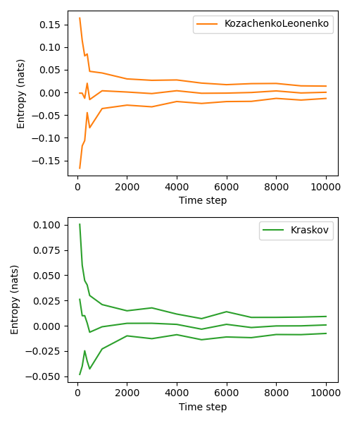
- Kraskov2004Kraskov, A., Stögbauer, H., & Grassberger, P. (2004). Estimating mutual information. Physical review E, 69(6), 066138.
- Charzyńska2016Charzyńska, A., & Gambin, A. (2016). Improvement of the k-NN entropy estimator with applications in systems biology. Entropy, 18(1), 13.
- KozachenkoLeonenko1987Kozachenko, L. F., & Leonenko, N. N. (1987). Sample estimate of the entropy of a random vector. Problemy Peredachi Informatsii, 23(2), 9-16.
- Charzyńska2016Charzyńska, A., & Gambin, A. (2016). Improvement of the k-NN entropy estimator with applications in systems biology. Entropy, 18(1), 13.