Usage and Applications
Example 1: Fractional nonlinear equation
\[D^\beta y(t) = \frac{40320}{\Gamma(9 - \beta)} t^{8 - \beta} - 3 \frac{\Gamma(5 + \beta / 2)}{\Gamma(5 - \beta / 2)} t^{4 - \beta / 2} + \frac{9}{4} \Gamma(\beta + 1) + \left( \frac{3}{2} t^{\beta / 2} - t^4 \right)^3 - \left[ y(t) \right]^{3 / 2}\]
For $0<\beta\leq1$ being subject to the initial condition $y(0)=0$, the exact solution is:
\[y(t)=t^8-3t^{4+\beta/2}+9/4t^\beta\]
# Inputs
tSpan = [0, 1];     # [intial time, final time]
y0 = 0;             # initial value
β = 0.9;            # order of the derivative

# ODE Model
par = β;
F(t, y, par) = (40320 ./ gamma(9 - par) .* t .^ (8 - par) .- 3 .* gamma(5 + par / 2)
           ./ gamma(5 - par / 2) .* t .^ (4 - par / 2) .+ 9/4 * gamma(par + 1) .+
           (3 / 2 .* t .^ (par / 2) .- t .^ 4) .^ 3 .- y .^ (3 / 2));

## Numerical solution
t, Yapp = FDEsolver(F, tSpan, y0, β, par);

# Plot
plot(t, Yapp, linewidth = 5, title = "Solution of a 1D fractional IVP",
     xaxis = "Time (t)", yaxis = "y(t)", label = "Approximation");
plot!(t, t -> (t.^8 - 3 * t .^ (4 + β / 2) + 9/4 * t.^β),
      lw = 3, ls = :dash, label = "Exact solution");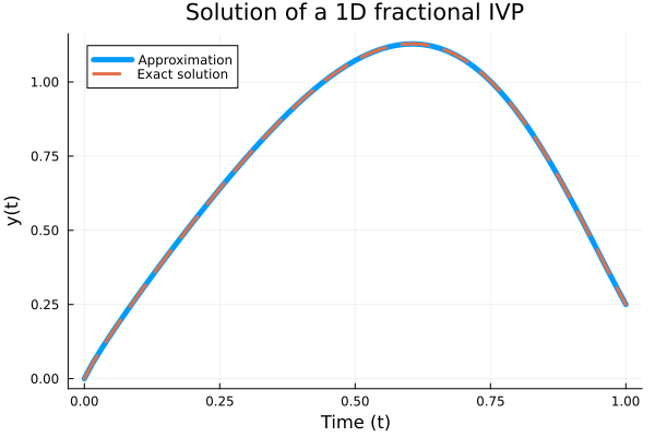
Example 2: Lotka-volterra-predator-prey
\[\begin{align*} D^{μ_1}u &= (\alpha - \beta v) u = \alpha u - \beta u v \\ D^{μ_2}v &= (-\gamma + \delta u) v = -\gamma v + \delta u v \end{align*}\]
# Inputs
tSpan = [0, 25];                    # [initial time, final time]
y0 = [34, 6];                       # initial values
μ = [0.98, 0.99];                # order of derivatives
par = [0.55, 0.028, 0.84, 0.026];   # model parameters

# ODE Model
function F(t, y, par)

    α = par[1]      # growth rate of the prey population
    β = par[2]      # rate of shrinkage relative to the product of the population sizes
    γ = par[3]       # shrinkage rate of the predator population
    δ = par[4]       # growth rate of the predator population as a factor of the product
                     # of the population sizes

    u = y[1]         # population size of the prey species at time t[n]
    v = y[2]         # population size of the predator species at time t[n]

    F1 = α .* u .- β .* u .* v
    F2 = - γ .* v .+ δ .* u .* v

    [F1, F2]

end

## Solution
t, Yapp = FDEsolver(F, tSpan, y0, μ, par);

# Plot
plot(t, Yapp, linewidth = 5, title = "Solution to LV model with 2 FDEs",
     xaxis = "Time (t)", yaxis = "y(t)", label = ["Prey" "Predator"]);
plot!(legendtitle = "Population of");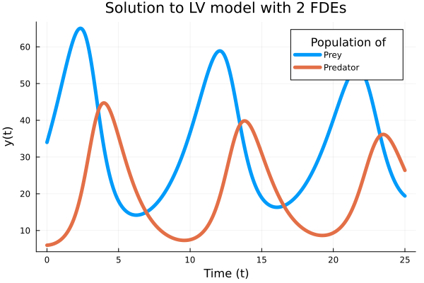
Example 3: SIR model
One application of using fractional calculus is taking into account effects of memory in modeling including epidemic evolution.
\[\begin{align*} D^{α_1}S &= -\beta IS, \\ D^{α_2}I &= \beta IS - \gamma I, \\ D^{α_3}R &= \gamma I. \end{align*}\]
By defining the Jacobian matrix, the user can achieve a faster convergence based on the modified Newton–Raphson method.
# Inputs
I0 = 0.001;             # intial value of infected
tSpan = [0, 100];       # [intial time, final time]
y0 = [1 - I0, I0, 0];   # initial values [S0,I0,R0]
α = [1, 1, 1];          # order of derivatives
h = 0.1;                # step size of computation (default = 0.01)
par = [0.4, 0.04];      # parameters [β, recovery rate]

## ODE model
function F(t, y, par)

    # parameters
    β = par[1]    # infection rate
    γ = par[2]    # recovery rate

    S = y[1]   # Susceptible
    I = y[2]   # Infectious
    R = y[3]   # Recovered

    # System equation
    dSdt = - β .* S .* I
    dIdt = β .* S .* I .- γ .* I
    dRdt = γ .* I

    return [dSdt, dIdt, dRdt]

end

## Jacobian of ODE system
function JacobF(t, y, par)

    # parameters
    β = par[1]     # infection rate
    γ = par[2]     # recovery rate

    S = y[1]    # Susceptible
    I = y[2]    # Infectious
    R = y[3]    # Recovered

    # System equation
    J11 = - β * I
    J12 = - β * S
    J13 =  0
    J21 =  β * I
    J22 =  β * S - γ
    J23 =  0
    J31 =  0
    J32 =  γ
    J33 =  0

    J = [J11 J12 J13
         J21 J22 J23
         J31 J32 J33]

    return J

end

## Solution
t, Yapp = FDEsolver(F, tSpan, y0, α, par, JF = JacobF, h = h);

# Plot
plot(t, Yapp, linewidth = 5, title = "Numerical solution of SIR model",
     xaxis = "Time (t)", yaxis = "SIR populations", label = ["Susceptible" "Infectious" "Recovered"]);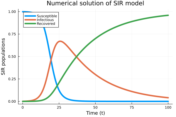
Example 4: Dynamics of interaction of N species microbial communities
The impact of ecological memory on the dynamics of interacting communities can be quantified by solving fractional form ODE systems.
\[D^{β_i}X_i = X_i \left( b_i f_i(\{X_k\}) - k_i X_i \right), \quad f_i(\{X_k\}) = \prod_{\substack{k=1 \\ k \neq i}}^N \frac{K_{ik}^n}{K_{ik}^n + X_k^n}.\]
tSpan = [0, 50];   # time span
h = 0.1;           # time step
N = 20;            # number of species
β = ones(N);       # order of derivatives
X0 = 2 * rand(N);  # initial abundances

# parametrisation
par = [5,
       rand(N),
       rand(N),
       2 * rand(N, N),
       N];

# ODE model
function F(t, x, par)

    l = par[1] # Hill coefficient
    b = par[2] # growth rates
    k = par[3] # death rates
    K = par[4] # inhibition matrix
    N = par[5] # number of species

    Fun = zeros(N)

    for i in 1:N

        # inhibition functions
        f = prod(K[i, 1:end .!= i] .^ l ./
             (K[i, 1:end .!= i] .^ l .+ x[ 1:end .!= i] .^l))

        # System of equations
        Fun[i] = x[ i] .* (b[i] .* f .- k[i] .* x[ i])

    end

    return Fun

end

# Solution
t, Xapp = FDEsolver(F, tSpan, X0, β, par, h = h, nc = 3, tol = 10e-9);

# Plot
plot(t, Xapp, linewidth = 5,
     title = "Dynamics of microbial interaction model",
     xaxis = "Time (t)");
     yaxis!("Log abundance", :log10, minorgrid = true);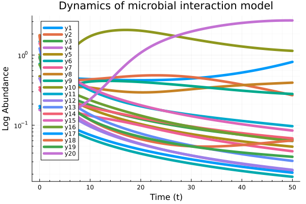
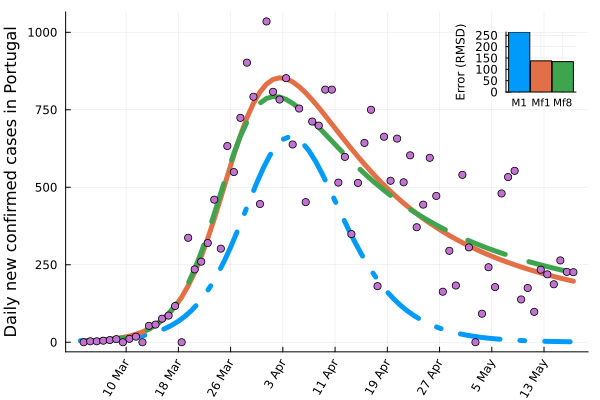
Example 5: Fitting orders of a COVID-19 model
Different methods are used to adjust the order of fractional differential equation models, which helps in analyzing systems across various fields.
We use Optim.jl to demonstrate how modifying system parameters and the order of derivatives in FdeSolver can enhance the fitting of COVID-19 data. The model is as follows:
\[\begin{align*} {D}_t^{\alpha_S} S(t) =& -\beta \frac{I}{N} S - l\beta \frac{H}{N} S - \beta' \frac{P}{N} S, \\ {D}_t^{\alpha_E} E(t) =& \beta \frac{I}{N} S + l\beta \frac{H}{N} S + \beta' \frac{P}{N} S - \kappa E, \\ {D}_t^{\alpha_I} I(t) =& \kappa \rho_1 E - (\gamma_a + \gamma_i) I - \delta_i I, \\ {D}_t^{\alpha_P} P(t) =& \kappa \rho_2 E - (\gamma_a + \gamma_i) P - \delta_p P, \\ {D}_t^{\alpha_A} A(t) =& \kappa (1 - \rho_1 - \rho_2) E, \\ {D}_t^{\alpha_H} H(t) =& \gamma_a (I + P) - \gamma_r H - \delta_h H, \\ {D}_t^{\alpha_R} R(t) =& \gamma_i (I + P) + \gamma_r H, \\ {D}_t^{\alpha_F} F(t) =& \delta_i I + \delta_p P + \delta_h H, \end{align*}\]
- Model M1: fits one parameter and uses integer orders.
- Model Mf1: fits one parameter, but adjusts the derivative orders; however, all orders are equal, representing a commensurate fractional order.
- Model Mf8: fits one parameter and allows for eight distinct derivative orders, accommodating incommensurate orders for more flexibility in modeling.
# Dataset subset
repo=HTTP.get("https://raw.githubusercontent.com/CSSEGISandData/COVID-19/master/csse_covid_19_data/csse_covid_19_time_series/time_series_covid19_confirmed_global.csv"); # dataset of Covid from CSSE
dataset_CC = CSV.read(repo.body, DataFrame); # all data of confirmed
Confirmed=dataset_CC[dataset_CC[!,2].=="Portugal",45:121]; #comulative confirmed data of Portugal from 3/2/20 to 5/17/20
C=diff(Float64.(Vector(Confirmed[1,:])));# Daily new confirmed cases

#preprocessing (map negative values to zero and remove outliers)
₋Ind=findall(C.<0);
C[₋Ind].=0.0;
outlier=findall(C.>1500);
C[outlier]=(C[outlier.-1]+C[outlier.-1])/2;

## System definition

# parameters
β=2.55; # Transmission coefficient from infected individuals
l=1.56; # Relative transmissibility of hospitalized patients
β′=7.65; # Transmission coefficient due to super-spreaders
κ=0.25; # Rate at which exposed become infectious
ρ₁=0.58; # Rate at which exposed people become infected I
ρ₂=0.001; # Rate at which exposed people become super-spreaders
γₐ=0.94; # Rate of being hospitalized
γᵢ=0.27; # Recovery rate without being hospitalized
γᵣ=0.5; # Recovery rate of hospitalized patients
δᵢ=1/23; # Disease induced death rate due to infected class
δₚ=1/23; # Disease induced death rate due to super-spreaders
δₕ=1/23; # Disease induced death rate due to hospitalized class
# Define SIR model
function SIR(t, u, par)
    # Model parameters.
	N, β, l, β′, κ,	ρ₁,	ρ₂,	γₐ,	γᵢ,	γᵣ,	δᵢ,	δₚ, δₕ=par

    # Current state.
    S, E, I, P, A, H, R, F = u

# ODE
    dS = - β * I * S/N - l * β * H * S/N - β′* P * S/N # susceptible individuals
    dE = β * I * S/N + l * β * H * S/N + β′ *P* S/N - κ * E # exposed individuals
    dI = κ * ρ₁ * E - (γₐ + γᵢ )*I - δᵢ * I #symptomatic and infectious individuals
    dP = κ* ρ₂ * E - (γₐ + γᵢ)*P - δₚ * P # super-spreaders individuals
    dA = κ *(1 - ρ₁ - ρ₂ )* E # infectious but asymptomatic individuals
	dH = γₐ *(I + P ) - γᵣ *H - δₕ *H # hospitalized individuals
	dR = γᵢ * (I + P ) + γᵣ* H # recovery individuals
	dF = δᵢ * I + δₚ* P + δₕ *H # dead individuals
    return [dS, dE, dI, dP, dA, dH, dR, dF]
end;

#initial conditions
N=10280000/875; # Population Size
S0=N-5; E0=0; I0=4; P0=1; A0=0; H0=0; R0=0; F0=0;
X0=[S0, E0, I0, P0, A0, H0, R0, F0]; # initial values
tspan=[1,length(C)]; # time span [initial time, final time]

par=[N, β,	l,	β′,	κ,	ρ₁,	ρ₂,	γₐ,	γᵢ,	γᵣ,	δᵢ,	δₚ, δₕ]; # parameters

## optimazation of β for integer order model

function loss_1(b) # loss function
	par[2]=b[1]
	_, x = FDEsolver(SIR, tspan, X0, ones(8), par, h = .1)
    appX=vec(sum(x[1:10:end,[3,4,6]], dims=2))
    rmsd(C, appX; normalize=:true) # Normalized root-mean-square error
end;

p_lo_1=[1.4]; #lower bound for β
p_up_1=[4.0]; # upper bound for β
p_vec_1=[2.5]; #  initial guess for β
Res1=optimize(loss_1,p_lo_1,p_up_1,p_vec_1,Fminbox(BFGS()),# Broyden–Fletcher–Goldfarb–Shanno algorithm
# Result=optimize(loss_1,p_lo_1,p_up_1,p_vec_1,SAMIN(rt=.99), # Simulated Annealing algorithm (sometimes it has better perfomance than (L-)BFGS)
			Optim.Options(outer_iterations = 10,
						  iterations=1000,
						  show_trace=false, # turn it true to see the optimization
						  show_every=1));
p1=vcat(Optim.minimizer(Res1));
par1=copy(par); par1[2]=p1[1];

## optimazation of β and order of commensurate fractional order model
function loss_F_1(pμ)
	par[2] = pμ[1] # infectivity rate
	μ = pμ[2] # order of derivatives

	_, x = FDEsolver(SIR, tspan, X0, μ*ones(8), par, h = .1)
    appX=vec(sum(x[1:10:end,[3,4,6]], dims=2))
    rmsd(C, appX; normalize=:true)
end;

p_lo_f_1=vcat(1.4,.5); # lower bound for β and orders
p_up_f_1=vcat(4,1); # upper bound for β and orders
p_vec_f_1=vcat(2.5,.9); #  initial guess for β and orders
ResF1=optimize(loss_F_1,p_lo_f_1,p_up_f_1,p_vec_f_1,Fminbox(LBFGS()), # LBFGS is suitable for large scale problems
# Result=optimize(loss,p_lo,p_up,pvec,SAMIN(rt=.99),
			Optim.Options(outer_iterations = 10,
						  iterations=1000,
						  show_trace=false, # turn it true to see the optimization
						  show_every=1));
pμ=vcat(Optim.minimizer(ResF1));
parf1=copy(par); parf1[2]=pμ[1]; μ1=pμ[2];

## optimazation of β and order of incommensurate fractional order model
function loss_F_8(pμ)
	par[2] = pμ[1] # infectivity rate
	μ = pμ[2:9] # order of derivatives
	if size(X0,2) != Int64(ceil(maximum(μ))) # to prevent any errors regarding orders higher than 1
		indx=findall(x-> x>1, μ)
		μ[indx]=ones(length(indx))
	end
	_, x = FDEsolver(SIR, tspan, X0, μ, par, h = .1)
    appX=vec(sum(x[1:10:end,[3,4,6]], dims=2))
    rmsd(C, appX; normalize=:true)
end;

p_lo=vcat(1.4,.5*ones(8)); # lower bound for β and orders
p_up=vcat(4,ones(8)); # upper bound for β and orders
pvec=vcat(2.5,.9*ones(8)); #  initial guess for β and orders
ResF8=optimize(loss_F_8,p_lo,p_up,pvec,Fminbox(LBFGS()), # LBFGS is suitable for large scale problems
# Result=optimize(loss,p_lo,p_up,pvec,SAMIN(rt=.99),
			Optim.Options(outer_iterations = 10,
						  iterations=1000,
						  show_trace=false, # turn it true to see the optimization
						  show_every=1));
pp=vcat(Optim.minimizer(ResF8));
parf8=copy(par); parf8[2]=pp[1]; μ8=pp[2:9];

## plotting
DateTick=Date(2020,3,3):Day(1):Date(2020,5,17);
DateTick2= Dates.format.(DateTick, "d u");

t1, x1 = FDEsolver(SIR, tspan, X0, ones(8), par1, h = .1); # solve ode model
_, xf1 = FDEsolver(SIR, tspan, X0, μ1*ones(8), parf1, h = .1); # solve commensurate fode model
_, xf8 = FDEsolver(SIR, tspan, X0, μ8, parf8, h = .1); # solve incommensurate fode model

X1=sum(x1[1:10:end,[3,4,6]], dims=2);
Xf1=sum(xf1[1:10:end,[3,4,6]], dims=2);
Xf8=sum(xf8[1:10:end,[3,4,6]], dims=2);

Err1=rmsd(C, vec(X1)); # RMSD for ode model
Errf1=rmsd(C, vec(Xf1)); # RMSD for commensurate fode model
Errf8=rmsd(C, vec(Xf8)); # RMSD for incommensurate fode model

plot(DateTick2,X1, ylabel="Daily new confirmed cases in Portugal",lw=5,
     label="M1",xrotation=rad2deg(pi/3), linestyle=:dashdot)
    plot!(Xf1, label="Mf1", lw=5)
    plot!(Xf8,  label="Mf8", linestyle=:dash, lw=5)
    scatter!(C, label= "Real data",legendposition=(.85,1),legend=:false)
	plPortugal=bar!(["M1" "Mf1" "Mf8"],[Err1 Errf1 Errf8], ylabel="Error (RMSD)",
		legend=:false, bar_width=2,yguidefontsize=8,xtickfontsize=7,
    inset = (bbox(0.04, 0.08, 70px, 60px, :right)),
    subplot = 2,
    bg_inside = nothing)