Examples
This section gives some examples for how this package can be used. In most of the examples that follow, there are exact solutions, but we do not discuss them here. You can see the scripts in the tests if you are interested.
Example I: Heat equation
We start with a simple example:
\[\begin{align*} \dfrac{\partial u}{\partial t} &= \dfrac{\partial^2 u}{\partial x^2}, \quad 0 < x < 1,\,t>0, \\[8pt] \dfrac{\partial u(0, t)}{\partial x} &= 0, \quad t>0, \\[8pt] \dfrac{\partial u(1, t)}{\partial x} &= 0, \quad t>0, \\[8pt] u(x, 0) & = x, \quad 0 < x < 1. \end{align*}\]
The first step is to define the geometry and the boundary conditions. The geometry for these types of problems simply requires a set of mesh_points, which can be regularly or irregular spaced. Here we use
mesh_points = LinRange(0, 1, 500)We could then use geo = FVMGeometry(mesh_points), but we will use the simpler constructor for the FVMProblem later. Note that the constructor will take $a=0$ and $b=1$ from mesh_points[begin] and mesh_points[end].
The boundary conditions are defined using the Neumann type. Since the boundary condition is constant in this case, we can use the simpler Neumann(::Number) constructor (see ?Neumann for other constructors).
using FiniteVolumeMethod1D
lhs = Neumann(0.0)
rhs = Neumann(0.0)
As before, we could then use BoundaryConditions(lhs, rhs), but we will use the simpler constructor for the FVMProblem. Now, let us define the diffusion function, initial condition, and final time.
diffusion_function = (u, x, t, p) -> one(u)
initial_condition = collect(mesh_points)
final_time = 0.1
We can now construct the FVMProblem.
prob = FVMProblem(mesh_points, lhs, rhs;
    diffusion_function,
    initial_condition,
    final_time)
This prob can be solved the same way as you would e.g. with DifferentialEquations.jl with solve. Using solve returns the same struct as DifferentialEquations.jl returns:
using OrdinaryDiffEq
using LinearSolve
sol = solve(prob, TRBDF2(linsolve=KLUFactorization()))
This can be easily plotted, e.g.
using CairoMakie
let t_range = LinRange(0.0, final_time, 250)
    fig = Figure(fontsize=33)
    ax = Axis(fig[1, 1], xlabel=L"x", ylabel=L"t")
    sol_u = [sol(t) for t in t_range]
    contourf!(ax, mesh_points, t_range, reduce(hcat, sol_u), colormap=:viridis)
    fig
end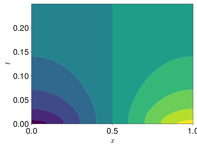
Example II: Reaction-diffusion equation
The next example we consider is a reaction-diffusion equation:
\[\begin{align*} \dfrac{\partial u}{\partial t} &= \dfrac{\partial^2 u}{\partial x^2} + \pi^2 \exp[-24\pi^2t]\sin(5\pi x), \quad 0 < x < 1,\, t > 0, \\[8pt] u(0, t) &= 0, \\[8pt] u(1, t) &= 0, \\[8pt] u(x, 0) &= 3\sin(4\pi x). \end{align*}\]
The boundary conditions can be constructed using Dirichlet. So, the geometry and boundary conditions can be given by:
using FiniteVolumeMethod1D
mesh_points = LinRange(0, 1, 500)
lhs = Dirichlet(0.0)
rhs = Dirichlet(0.0)
Now, let us define the diffusion and reaction functions. We show here the use of parameters.
diffusion_function = (u, x, t, p) -> one(u)
reaction_function = (u, x, t, p) -> p[1] * exp(-p[2] * t) * sin(p[3] * x)
reaction_parameters = (π^2, 24π^2, 5π)
Now the problem can be constructed.
ic_ff = x -> 3sin(4π*x)
initial_condition = ic_ff.(mesh_points)
final_time = 0.05
prob = FVMProblem(mesh_points, lhs, rhs;
    diffusion_function,
    reaction_function,
    reaction_parameters,
    initial_condition,
    final_time)
Now we solve and plot the solution.
using OrdinaryDiffEq
using LinearSolve
sol = solve(prob, TRBDF2(linsolve=KLUFactorization()), saveat = 0.001)

using CairoMakie
let t_range = LinRange(0.0, final_time, 250)
    fig = Figure(fontsize=33)
    ax = Axis3(fig[1, 1], xlabel=L"x", ylabel=L"t", zlabel=L"z", azimuth = 0.8)
    sol_u = [sol(t) for t in t_range]
    surface!(ax, mesh_points, t_range, reduce(hcat, sol_u), colormap=:viridis)
    fig
end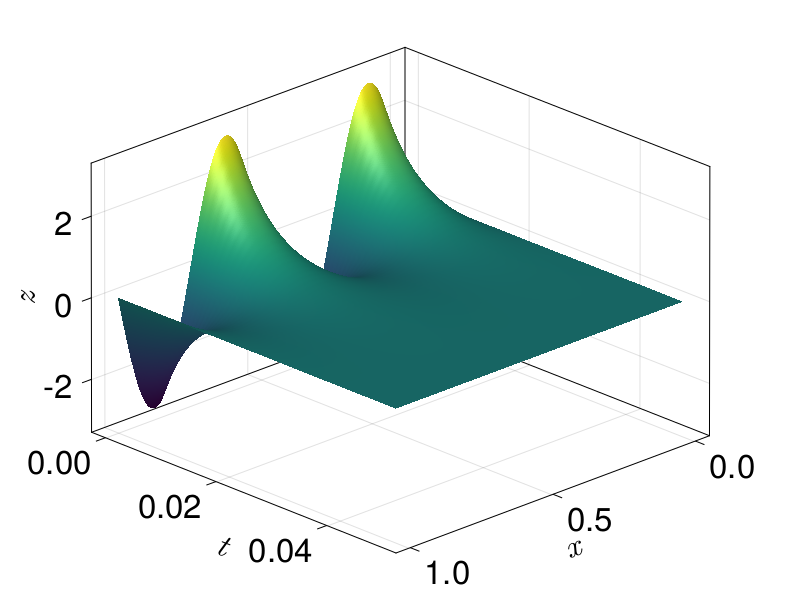
Example III: Diffusion problem with Robin boundary conditions
This next problem we consider is a diffusion problem with Robin boundary conditions:
\[\begin{align*} \dfrac{\partial u}{\partial t} & = \frac{1}{25}\dfrac{\partial^2 u}{\partial x^2}, \quad 0 < x < 3,\, t>0, \\[8pt] u(0, t) & = 0, \\[8pt] \dfrac{1}{2}u(3, t) + \dfrac{\partial u(3, t)}{\partial x} &= 0,\\[8pt] u(x, 0) & = 100\left(1-\dfrac{x}{3}\right). \end{align*}\]
Robin boundary conditions are supported by rewriting them in Neumann form, so that $\partial u(3, t)/\partial x = -u(3, t)/2$ in the above. Thus:
using FiniteVolumeMethod1D
mesh_points = LinRange(0, 3, 2500)
lhs = Dirichlet(0.0)
rhs = Neumann((u, t, p) -> u * p, -1 / 2)
diffusion_function = (u, x, t, p) -> p^2
diffusion_parameters = 1 / 5
ic = x -> 100(1 - x / 3)
initial_condition = ic.(mesh_points)
final_time = 3.0
prob = FVMProblem(mesh_points, lhs, rhs;
    diffusion_function,
    diffusion_parameters,
    final_time=final_time,
    initial_condition
)

using OrdinaryDiffEq
using LinearSolve
sol = solve(prob, TRBDF2(linsolve=KLUFactorization()), saveat = 0.01)

using CairoMakie
let t_range = LinRange(0.0, final_time, 250)
    fig = Figure(fontsize=33)
    ax = Axis3(fig[1, 1], xlabel=L"x", ylabel=L"t", zlabel=L"z", azimuth = 0.8)
    sol_u = [sol(t) for t in t_range]
    surface!(ax, mesh_points, t_range, reduce(hcat, sol_u), colormap=:viridis)
    fig
end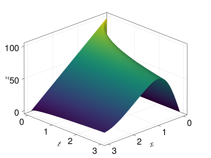
Example IV: Porous-Fisher equation with degenerate diffusion
We now consider the following problem:
\[\begin{align*} \dfrac{\partial u}{\partial t} &= \dfrac{\partial}{\partial x}\left(D(u)\dfrac{\partial u}{\partial x}\right) + R(u), \quad -6\pi < x < 6\pi,\\[8pt] \dfrac{\partial u(-2\pi, t)}{\partial x} & = 0, \\[8pt] \dfrac{\partial u(2\pi, t)}{\partial x} & = 0, \\[8pt] u(x, 0) & = \begin{cases} 1 & x < 0, \\ 1/2 & x \geq 0, \end{cases} \end{align*}\]
where $D(u) = 1/(10u) + 50/u^2 + 3/u^3$ and $R(u) = \beta K u(1 - u/K)$. We take $\beta = 10^{-3}$ and $K = 2$. The problem is solved as follows:
using FiniteVolumeMethod1D
mesh_points = LinRange(-2π, 2π, 500)
lhs = Neumann(0.0)
rhs = Neumann(0.0)
diffusion_function = (u, x, t, p) -> inv(p[1] * u) + p[2] * inv(u^2) + p[3] * inv(u^3)
diffusion_parameters = [1.0, 50.0, 3.0]
reaction_function = (u, x, t, p) -> p[1] * p[2] * u * (1 - u / p[2])
reaction_parameters = [1e-3, 2.0]
ic_f(x) = x < 0 ? 1.0 : 1 / 2
initial_condition = ic_f.(mesh_points)
final_time = 1.0
prob = FVMProblem(
    mesh_points,
    lhs,
    rhs;
    diffusion_function,
    reaction_function,
    diffusion_parameters,
    reaction_parameters,
    initial_condition,
    final_time
)

using OrdinaryDiffEq
sol = solve(fvm_prob, TRBDF2())

using CairoMakie
let t_range = LinRange(0.0, final_time, 250)
    fig = Figure(fontsize=33)
    ax = Axis3(fig[1, 1], xlabel=L"x", ylabel=L"t", zlabel=L"z", azimuth = 0.8)
    sol_u = [sol(t) for t in t_range]
    surface!(ax, mesh_points, t_range, reduce(hcat, sol_u), colormap=:viridis)
    fig
end