QTL analysis

This section describes a step-by-step guide for QTL analysis.

Input data file format

The package FlxQTL does not require any particular data format. Any file readable in Julia is fine, but the input should contain traits (or phenotypes), genotype (probability), marker information on marker names, chromosomes, and marker positions, and optionally climatic information. All inputs are types of Arrays in Julia and should have no missing values, i.e. imputation is required if missing values exist.

Reading the data files and processing arrays

Use any Julia package able to read data files (.txt, .csv, etc.). Julia's built-in module DelimitedFiles supports read, and write files. Let's try using an example dataset in FlxQTL. It is plant data: Arabidopsis thaliana in the data folder. Detailed description on the data can be referred to README in the folder.

using DelimitedFiles

pheno = readdlm("data/Arabidopsis_fitness.csv",',';skipstart=1); # skip to read the first row (column names) to obtain a matrix only

geno = readdlm("data/Arabidopsis_genotypes.csv",',';skipstart=1); 

markerinfo = readdlm("data/Arabidopsis_markerinfo_1d.csv",',';skipstart=1);

For efficient computation, the normalization of matrices is necessary. The phenotype matrix labelled as pheno here composes of wide range of values from 1.774 to 34.133, so that it is better to narow the range of values in [0,1], [-1,1], or any narrower interval for easy computation. Note that the dimension of a phenotype matrix should be the number of traits x the number of individuals.

using Statistics, StatsBase
Y=convert(Array{Float64,2},pheno'); #convert from transposed one to a Float64 matrix
Ystd=(Y.-mean(Y,dims=2))./std(Y,dims=2); # sitewise normalization

!!! Note

• If the data are skewed or have outliers, simple standadization may not resolve them. You may use a Y_huber function to rescale the data to be less sensitve to outliers.

In the genotype data, 1, 2 indicate Italian, Swedish parents, respectively. You can rescale the genotypes for efficiency.

geno[geno.==1.0].=0.0;geno[geno.==2.0].=1.0; # or can do geno[geno.==1.0].=-1.0 for only genome scan

For genome scan, we need restructure the standardized genotype matrix combined with marker information. Note that the genome scan in FlxQTL is implemented by CPU parallelization, so we need to add workers (or processes) before the genome scan. Depending on the computer CPU, one can add as many processes as possible. If your computer has 16 cores, then you can add 15 or little more. Note that you need to type @everywhere followed by using PackageName for parallel computing. The dimension of a genotype (probability) matrix should be the number of markers x the number of individuals.

using Distributed
addprocs(4) 
@everywhere using FlxQTL 
XX=Markers(markerinfo[:,1],markerinfo[:,2],markerinfo[:,3],geno') # marker names, chromosomes, marker positions, genotypes

• Julia tip: Whenever you reload a package, i.e. using FlxQTL, you should re-enter XX=FlxQTL.Markers(markerinfo[:,1],markerinfo[:,2],markerinfo[:,3],geno') to fresh the struct of array. If not, your genome scan throws an error. You should also do with another struct of array in a submodule QTLplot, FlxQTL.layers.

Optionally, one can generate a trait covariate matrix (Z). The first column indicates overall mean between the two regions, and the second implies site difference: -1 for Italy, and 1 for Sweden.

Z=hcat(ones(6),vcat(-ones(3),ones(3)))
m,q = size(Z) # check the dimension

Computing a genetic (or climatic) relatedness matrix

The submodule GRM contains functions for computing kinship matrices, kinshipMan, kinship4way, kinshipGs, kinshipLin, kinshipCtr, and computing 3D array of kinship matrices for LOCO (Leave One Chromosome Out) with a shrinkage method for nonpositive definiteness, shrinkg, shrinkgLoco, kinshipLoco. Note that the shrinkage option is only used for kinshipMan, kinship4way.

For the Arabidopsis genotype data, we will use a genetic relatedness matrix using manhattan distance measure, kinshipMan with a shrinkage with the LOCO option.

Kg = shrinkgLoco(kinshipMan,10,XX)

For no LOCO option with shrinkage,

K = shrinkg(kinshipMan,10,XX.X)

If you have climatic information on your trait data, you can compute the relatedness matrix using one of the above functions, but it is recommended using kinshipGs,kinshipLin,kinshipCtr after normalization. Since the climatic information is not available, we use an identity matrix.

using LinearAlgebra
Kc = Matrix(1.0I,6,6) # 3 years x 2 sites

1D genome scan

Once all input matrices are ready, we need to proceed the eigen-decomposition to two relatedness matrices. For a non-identity climatic relatedness, and a kinship with LOCO, you can do eigen-decomposition simultaneously. Since we use the identity climatic relatedness, you can use Matrix(1.0I,6,6) for a matrix of eigenvectors and ones(6) for a vector of eigenvalues.

Tg,Λg,Tc,λc = K2Eig(Kg,Kc,true); # the last argument: LOCO::Bool = false (default)

Tg,λg = K2eig(Kg, true) # for eigen decomposition to one kinship with LOCO

For eigen decomposition to one kinship with no LOCO option,

T,λ = K2eig(K)

Now start with 1D genome scan with (or without) LOCO including Z or not. For the genome scan with LOCO including Z,

LODs,B,est0 = geneScan(1,Tg,Tc,Λg,λc,Ystd,XX,Z,true); # FlxQTL for including Z (trait covariates) or Z=I

For the genome scan with LOCO excluding Z, i.e. an identity matrix, we have two options: a FlxQTL model and a conventional MLMM

LODs,B,est0 = geneScan(1,Tg,Tc,Λg,λc,Ystd,XX,true); # FlxQTL for Z=I 

LODs,B,est0 = geneScan(1,Tg,Λg,Ystd,XX,true); # MLMM

Note that the first argument in geneScan is cross::Int64, which indicates a type of genotype or genotype probability. For instance, if you use a genotype matrix whose entry is one of 0,1,2, type 1. If you use genotype probability matrices, depending on the number of alleles or genotypes in a marker, one can type the corresponding number. i.e. 4-way cross: 4, HS DO mouse: 8 for alleles, 32 for genotypes, etc.

For no LOCO option,

LODs,B,est0 = geneScan(1,T,Tc,λ,λc,Ystd,XX,Z);

LODs,B,est0 = geneScan(1,T,Tc,λ,λc,Ystd,XX);

LODs,B,est0 = geneScan(1,T,λ,Ystd,XX); # MLMM

The function geneScan has three arguments: LOD scores (LODs), effects matrix under H1 (B), and parameter estimates under H0 (est0), which is an Array{Any,1}. If you want to see null parameter esitmate in chromosome 1 for LOCO option, type est0[1].B, est0[1].loglik, est0[1].τ2, est0[1].Σ. In particular, you can extract values from each matrix in B (3D array of matrices) to generate an effects plot. To print an effect size matrix for the third marker, type B[:,:,3].

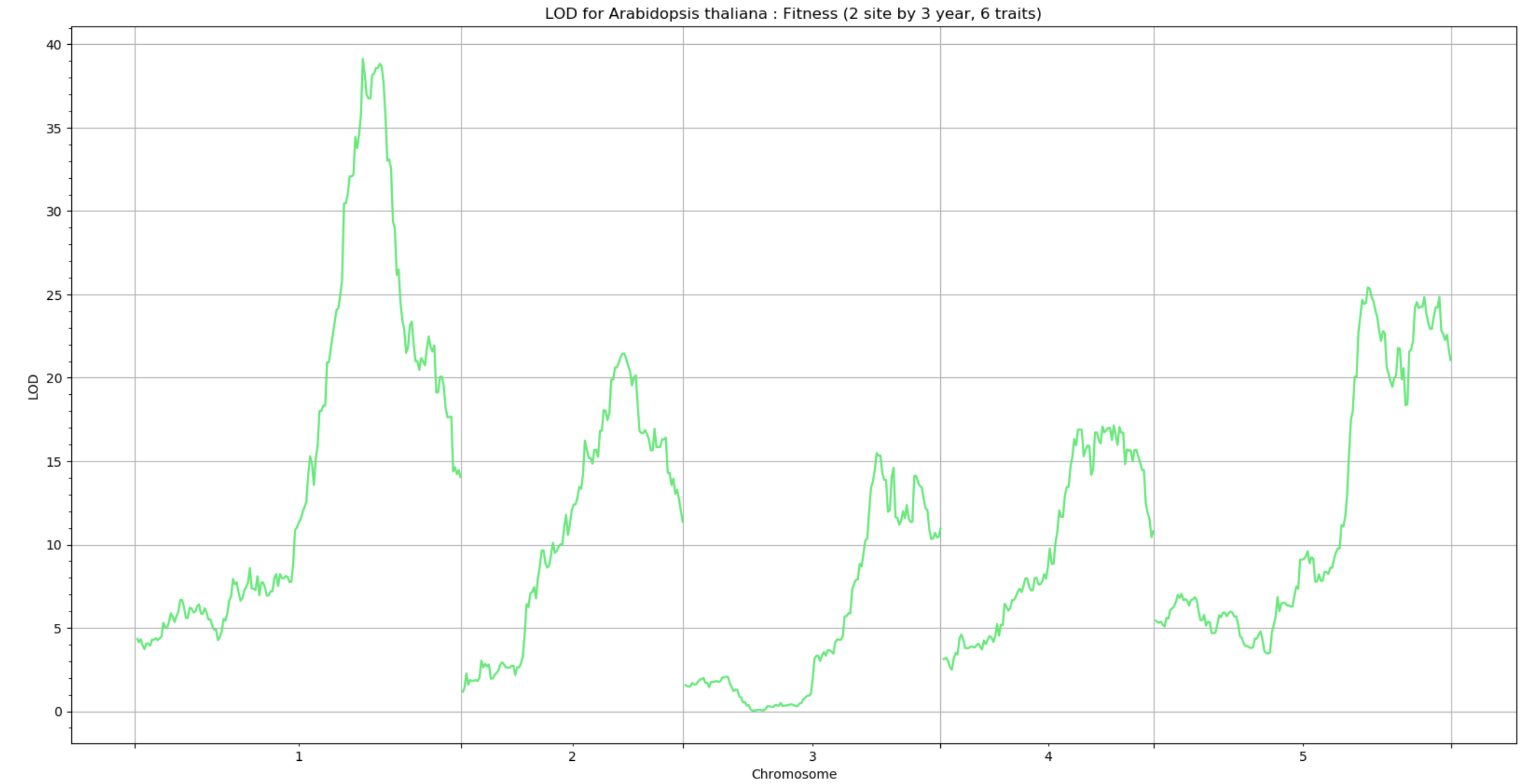
Generating plots

The QTLplot module is currently unavailable but plotting functions will be replaced with BigRiverQTLPlots.jl soon.

Performing a permutation test

Since the statistical inference for FlxQTL relies on LOD scores and LOD scores, the function permTest finds thresholds for a type I error. The first argument is nperm::Int64 to set the number of permutations for the test. For Z = I, type Matrix(1.0I,6,6) for the Arabidopsis thaliana data. In the keyword argument, pval=[0.05 0.01] is default to get thresholds of type I error rates (α). Note that permutation test is implemented by no LOCO option.

maxLODs, H1par_perm, cutoff = permTest(1000,1,K,Kc,Ystd,XX,Z;pval=[0.05]) # cutoff at 5 %