FrequencySweep.jl
Welcome to the FrequencySweep.jl's documentation! The FrequencySweep.jl library is targeted at the estimation of frequency response functions for systems of differential equations where the analytical representation is difficult to obtain.
The primary concept behind the operation of this library is rather straight forward. It is assumed that the solution to the user-defined system of differential equations can be obtained numerically for a specified oscillation frequency of a harmonic forcing function. It is also assumed that the solution at each frequency point will eventually tend towards a steady-state response where any transient behavior has decayed to such a point as to be irrelevant. Once this steady-state condition is obtained the FrequencySweep library simply determines the amplitude and phase of the solution. The final conditions of the solution at a particular frequency point are used as the initial conditions for the next frequency point thereby providing a frequency sweeping behavior. This sweeping behavior is oftentimes necessary to observe interesting nonlinear phenomenon such as jump phenomenon. A classical system illustrating jump phenomenon is the Duffing equation. The frf_sweep function is used to numerically estimate the frequency response functions.
frf_sweep
FrequencySweep.frf_sweep — Functionrst = frf_sweep(fcn, init, freq)
Description
The frf_sweep function computes the frequency response functions for a system of ordinary differential equations (ODE's) by means of "sweeping" across a range of excitation frequencies. The algorithm solves the system of ODE's at each excitation frequency in the supplied range. It uses the solution of these equations to determine the amplitude and phase of the resulting wavefuorm once it has sufficiently damped out the transient component of the solution. The amplitude and phase are determined by a discrete Fourier transform of the last N cycles of the solution waveform for each ODE.
Arguments
fcn: The solver requires the user to define a function supplying the ODE's to integrate. This function must be defined as follows.
function fcn(du, u, p, omega, t)
    # User code goes here
end
The arguments to the function are as follows:
- du: This is an output array where the output of each first order equation should be written.
- u: This is an input array the same size as du providing the current estimates for each state variable.
- p: A structure of user-defined type that can be used to pass model parameters.
- f: The oscillation frequency the solver is analyzing. This value will be supplied in the same units as supplied by the user.
- t: The independent variable, typically time.
init: The user must also supply an initial set of initial conditions for the solution of the ODE's. This set of initial conditions is only used for the solution to the first frequency value in the range as the solver will update the initial condition vector for subsequent frequency value solutions.
freq: The user must also supply a range of frequency values at which to compute the frequency responses. Ensure that there are no zero-valued frequencies in the range as the solver does not accept such a value. The solver utilizes the frequency value as a method of determining the length of the ODE solution; therefore, smaller frequency values result in longer solutions. A note about units: It is recommended that the frequency values be supplied with units of radians per unit time; however, whatever units are provided will be the same units used for the value passed to fcn.
The function returns a named tuple with two fields:
- frequency: An M-element array containing the frequency points at which the solution was computed.
- response: An M-by-N matrix where M is the number of frequency points and N is the number of ODE's being solved. The result is complex-valued such that each column of the matrix describes both the amplitude and phase of each equation.
The user may supply a set of optional parameters to control both the ODE solver and the calculation of amplitude and phase for each equation. The optional parameters are as follows.
ODE Solver Optional Arguments
- alg_hints: Any hints to pass to the ODE solver (e.g. :stiff).
- reltol: The relative solution tolerance.
- abstol: The absolute solution tolerance.
- dtmax: The maximum allowable step size in the independent variable.
- maxiters: The maximum number of iterations to allow.
- modelparams: A container for arguments to pass to fcn.
- solver: The ODE solver to utilize. The default is Tsit5(). See DifferentialEquations.jl for all available solvers.
Additional Optional Arguments
- pointspercycle: Defines the number of solution points for each cycle of the solution.
- cyclecount: Defines the number of solutions to use in the calculation of the amplitude and phase.
- transientcount: Defines how many cycles to let pass for the transient to sufficiently decay.
- windowsize: Defines the size of window to utilize for the discrete Fourier transform.
- windowfunction: Defines the window function to utilize for the discrete Fourier transform. The function should take the same form as the windowing functions from the DSP.jl library.
- zerotol: Provides a tolerance of closeness to zero for frequency values. Frequency values whose magnitude is below this threshold are ignored during the analysis.
frf_sweep Example
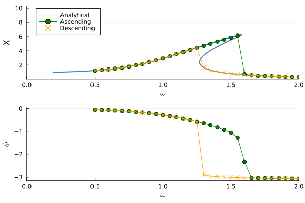
The following example illustrates how to use the function to obtain both an ascending and descending solution to Duffing's equation.
# Duffing's Equation
function duffing_eqn(du, u, p, omega, t)
    du[1] = u[2]
    du[2] = gamma * cos(omega * t) - delta * u[2] - alpha * u[1] - beta * u[1]^3
end

# Frequency Points
f1 = 0.5:0.05:2.0
f2 = 2.0:-0.05:0.5

# Perform the sweep
sweep1 = frf_sweep(
    duffing_eqn,
    [0.0, 0.0],
    f1
)
sweep2 = frf_sweep(
    duffing_eqn,
    [0.0, 0.0],
    f2
)
The solution returned from frf_sweep is an M-by-N matrix where M is the number of frequency points and N is the number of equations defined. The solution is complex-valued such that each column supplies both magnitude and phase information for each equation. For the Duffing model utilized above, the frequency response of the first equation is as follows.

Chirp Routines
The FrequencySweep.jl library also exposes routines to compute variable frequency signals often referred to as chirp signals. The library exposes routines to compute the signal, its first time derivative, and its second time derivative.
FrequencySweep.linear_chirp — TypeDescription
A linear chirp is a chirp signal whose frequency varies linearly with time. A linear chirp is given by the following function. $x(t) = X \sin \left( \left( \frac{ \left(f_{1} - f_{0} \right) t^2}{2 t_{span}} + f_{0} t \right) + \phi \right)$
Members
- amplitude: The amplitude of the signal.
- start_frequency: The initial frequency with units of rad/s, assuming time units of seconds of course.
- end_frequency: The final frequency with units of rad/s, assuming time units of seconds of course.
- time_span: The time duration over which the frequency will transition between the starting and ending frequencies.
- phase: The phase lag of the signal, in radians.
FrequencySweep.exponential_chirp — TypeDescription
An exponential chirp is a chirp signal whose frequency varies exponentially with time. An exponential chirp is given by the following function.
\[x(t) = X \sin \left( f_{0} \left( \frac{k^t - 1}{\ln (k)} \right) + \phi \right)\]
Where
\[k = \left( \frac{f_1}{f_0} \right)^{1/t_{span}}\]
Members
- amplitude: The amplitude of the signal.
- start_frequency: The initial frequency with units of rad/s, assuming time units of seconds of course.
- end_frequency: The final frequency with units of rad/s, assuming time units of seconds of course.
- time_span: The time duration over which the frequency will transition between the starting and ending frequencies.
- phase: The phase lag of the signal, in radians.
FrequencySweep.hyperbolic_chirp — TypeDescription
A hyperbolic chirp is a chirp signal whose frequency varies hyperbolically with time. A hyperbolic chirp is given by the following function.
\[x(t) = X \sin \left( \alpha \ln \left( 1 - \beta t \right) + \phi \right)\]
Where
\[\alpha = -\frac{f_0 f_1 t_{span}}{f_1 - f_0}\]
and
\[\beta = \frac{f_1 - f_0}{f_1 t_{span}}\]
Members
- amplitude: The amplitude of the signal.
- start_frequency: The initial frequency with units of rad/s, assuming time units of seconds of course.
- end_frequency: The final frequency with units of rad/s, assuming time units of seconds of course.
- time_span: The time duration over which the frequency will transition between the starting and ending frequencies.
- phase: The phase lag of the signal, in radians.
FrequencySweep.f — Functionrst = f(c, t)
Description
Evaluates a linear chirp signal at time t.
Arguments
- c: The linear_chirp instance.
- t: The time at which to evaluate the function.
rst = f(c, t)
Description
Evaluates an exponential chirp signal at time t.
Arguments
- c: The exponential_chirp instance.
- t: The time at which to evaluate the function.
rst = f(c, t)
Description
Evaluates a hyperbolic chirp signal at time t.
Arguments
- c: The hyperbolic_chirp instance.
- t: The time at which to evaluate the function.
FrequencySweep.df — Functionrst = df(c, t)
Description
Evaluates the first time derivative of a linear chirp signal at time t.
Arguments
- c: The linear_chirp instance.
- t: The time at which to evaluate the function.
rst = df(c, t)
Description
Evaluates the first time derivative of an exponential chirp signal at time t.
Arguments
- c: The exponential_chirp instance.
- t: The time at which to evaluate the function.
rst = df(c, t)
Description
Evaluates the first time derivative of a hyperbolic chirp signal at time t.
Arguments
- c: The hyperbolic_chirp instance.
- t: The time at which to evaluate the function.
FrequencySweep.df2 — Functionrst = df2(c, t)
Description
Evaluates the second time derivative of a linear chirp signal at time t.
Arguments
- c: The linear_chirp instance.
- t: The time at which to evaluate the function.
rst = df2(c, t)
Description
Evaluates the second time derivative of an exponential chirp signal at time t.
Arguments
- c: The exponential_chirp instance.
- t: The time at which to evaluate the function.
rst = df2(c, t)
Description
Evaluates the second time derivative of a hyperbolic chirp signal at time t.
Arguments
- c: The hyperbolic_chirp instance.
- t: The time at which to evaluate the function.
Chirp Example
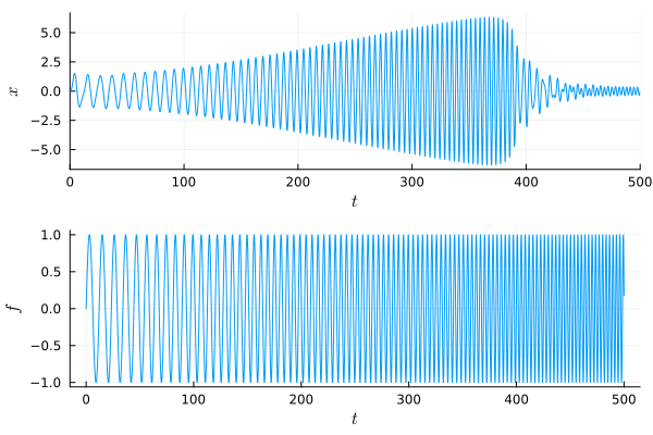
The following example illustrates the use of the chirp routines for the same Duffing model used in the frf_sweep example.
# Define a linear chirp
lc = linear_chirp(
    1.0,
    0.5,
    2.0,
    500.0,
    0.0
)

# Duffing Model Parameters
# x" + delta * x' + alpha * x + beta * x^3 = gamma * cos(omega * t)
alpha = 1.0
gamma = 1.0
delta = 0.1
beta = 0.05

# Duffing's Equation
function duffing_eqn(du, u, p, t)
    du[1] = u[2]
    du[2] = gamma * f(lc, t) - delta * u[2] - alpha * u[1] - beta * u[1]^3
end

# Solve the model
prob = ODEProblem(duffing_eqn, [0.0, 0.0], [0.0, lc.time_span])
sol = solve(prob)