FvCFD.jl is a simple explicit compressible Euler solver for 3D unstructured polyhedral meshes. The code is compact enough to be read fully by individual users/developers (<2000 lines) and makes for an excellent hands-on introduction to CFD. This code was originally a final project for a graduate numerical methods class, and would be a good starting point for additional projects or low-overhead numerical research.
| Property | Value |
|---|---|
| Mesh format | OpenFOAM |
| Output format | .vtu solution + ascii restart files |
| Convective schemes | JST & MUSCL+Roe |
| Gradient schemes | Green-Gauss & Weighted Least-Squares |
| Time discretization (transient) | Explicit Runge-Kutta orders 1-4 |
| Time discretization (steady-state) | Explicit first-order local time-stepping |
| Dependencies | WriteVTK |
Ongoing projects include the implementation of adaptive meshing and implicit time-stepping. All contributions are welcome.
To get started, use the instructions below to install FvCFD and run the included example cases. For developers, look at dataStructuresDefinitions.md to get familiar with the data structures used to represent the mesh and current solution in FvCFD.jl.
Install
- Start Julia:
$ julia - Activate the Julia package manager:
julia> ] - Either:
a. (Recommended) install Julia package:pkg> add FvCFD
b. OR install directly from GitHub:pkg> add https://github.com/henrystoldt/FvCFD.git
c. OR activate local copy of the code (must run Julia in this repository's main directory):pkg> activate . - (Optional) run tests to ensure the installation worked:
pkg> test FvCFD - Press backspace to exit the package manager
Run example cases
Example scripts to run simple included cases are stored in ./Examples
To run one:
- Clone this repository somewhere convenient:
$ git clone https://github.com/henrystoldt/FvCFD.git - Start Julia from in main directory of this git repository (same location where this file is stored):
$ julia - Execute the example script for the case you'd like to run:
julia> include("./Examples/shockTube.jl") - After the simulation completes, view the solution.xx.vtu files that were created using a post-processing tool like Paraview
Sample results
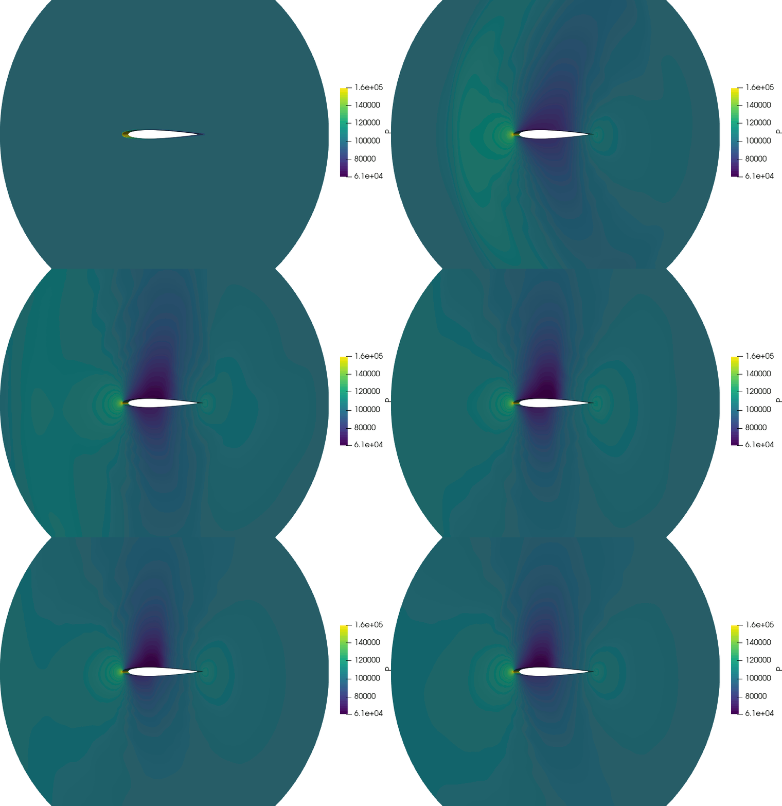
Forward step/Title animation: Mach 3 forward step problem (transient, 2D, quadratic uniform mesh), third-order Shu-Osher time-stepping CFL=0.5, JST convective discretization.
Case is originally from Woodward & Collela (1984), OpenFOAM comparison results available in Greenshields et al. (2010).
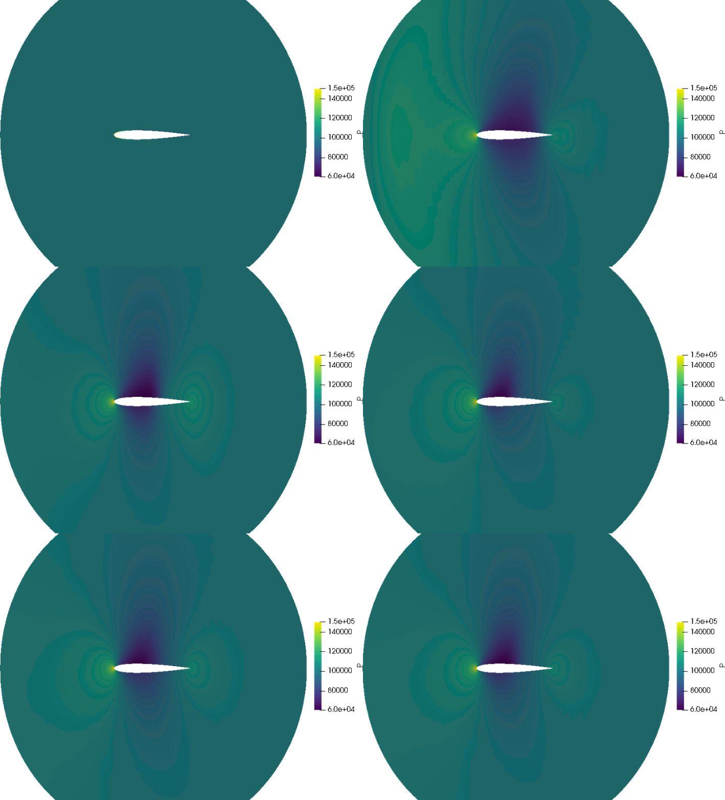
Transonic NACA 0012: Mach 0.8, AOA 1.25 degrees, Euler time integration, JST convective discretization

Transonic NACA 0012: Same as above but using local time-stepping. Note that although the animation speeds look similar, they do not correspond to equal amounts of computational time. Each frame in the animation above (global time-stepping) corresponds to 185 solver iterations, while each frame in the animation below (local time-stepping) corresponds to 20 solver iterations.

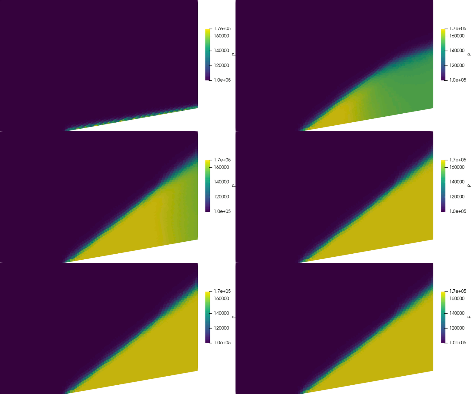
Supersonic wedge: Mach 2, 10 degree ramp angle, triangular mesh, Euler time integration, JST convective discretization. Properties correspond to one of the SU2 tutorial cases.

Mesh Compatibility Note
If you are getting errors trying to load an OpenFOAM mesh, try running the mesh through OpenFOAM's renumberMesh utility to standardize its formatting:
$ renumberMesh -overwrite (execute inside OpenFOAM case directory, then use the new mesh files generated in ./constant/polyMesh)
This can be helpful because FvCFD's current mesh parser is less flexible than OpenFOAM's. If you're interested in improving this, have a look at the readOF*File functions in mesh.jl. Should be fairly straightforward to improve these functions to accept whatever variation of the OF mesh format your meshing tool is generating.
(Developers) Running tests on local copy of the code
- Start Julia (In main git directory):
$ julia - Enter package manager:
julia> ] - Activate current directory's environment
pkg> activate . - Run tests:
pkg> test FvCFD
All of the tests are defined in files named ./test/test_*.jl. You can add new tests to the existing files or create new ones that follow that naming pattern (ex. ./test/test_MyNewCode.jl). Tests are discovered/run by ./test/runtests.jl, which is what pkg runs when you tell it to test FvCFD.
For newcomers to Julia
Julia is a dynamically-typed language that makes extensive use of Just-in-Time Compilation (JIT). In scientific computing, this approach can often deliver something approximating the speed of C++ combined with the simplicity of Python. Unfortunately, since compilation and execution are mixed together, Julia's speed is not always immediately obvious.
Compilation (Julia user experience)
The first time you execute a piece of code Julia performs type-inference, compiles any code for which it is able to infer types, and then runs it. As a result, it often takes longer than you would expect to run code for the first time (compared to languages like Python). Fortunately, after you've run code once, instances of Julia will cache the compiled code and will only need to recompile parts that you change, making subsequent runs much faster. To take advantage of this, you can start an instance of Julia and run your code in it repeatedly, without closing the REPL.
However, this can also cause problems in that any function that has been executed/compiled in an instance of Julia remains cached and available for use until the REPL is closed. As such, instances of Julia are stateful. This can lead to unexpected/non-replicable behavior in your code if it uses an old or deleted function which would not be present in a brand new instance of Julia executing your code. Check for these problems by restarting Julia and running your code/tests from scratch every so often or after significant changes.
Type-Stability (Julia developer experience)
Delving into the previous topic a bit more, Julia can execute your code in two distinct ways: compiled or not-compiled/interpreted. As you can imagine, executing compiled code is orders of magnitude faster than interpreting code and Julia will compile any code it can to take advantage of this. As such, the first and most important step to writing high performance Julia code is to ensure that Julia can compile it.
To be able to compile code, Julia needs to know the types of all variables involved at all times. This allows Julia to both allocate the appropriate amount of memory for each variable, and (later) to understand/interpret the data stored there. Julia can infer most variable types and does not need type annotations everywhere, with type inference. Whenever possible, make sure functions return variables of a consistent type (a type-stable function). Similarly, avoid changing the types of variables within functions - keep variables 'type-stable'. Use Julia's @code-warntype macro to check for type-stability problems.
A common workflow is to start by a creating an prototype without worrying excessively about type stability or performance, resulting in code similar to Python. Then, as/if the project progresses, the code's speed can be increased dramatically by adding a few type annotations and minor refactoring, without having to rewrite it in another language.
More information about Julia: https://julialang.org/
General documentation: https://docs.julialang.org/en/v1/
Julia performance tips: https://docs.julialang.org/en/v1/manual/performance-tips/
Julia/general performance tips: https://biojulia.net/post/hardware/
Nomenclature
For the simple variables:
| Var | Meaning | Units |
|---|---|---|
| e | internal energy | J/kg |
| P | Pressure | Pa |
| rho | Density | kg/m^3 |
| T | Temperature | K |
| U | Velocity | m/s |
And the state & flux variables:
| Var | Meaning | Definition |
|---|---|---|
| xMom | x-Momentum | rho*U |
| eV2 | total energy | rho*(e + U^2/2) |
| rhoU2p | flux of x-momentum | rho*U^2 + P |
| rhoUeV2PU | x-direction flux of total energy | UeV2 + PU |
References
These are referred to throughout the code:
Moukalled et al.: The Finite Volume Method in Computational Fluid Dynamics: An Advanced Introduction with OpenFOAM and Matlab
Hoffman: Numerical Methods for Engineers and Scientists
Versteeg et al.: An Introduction to Computational Fluid Dynamics: The Finite Volume Method (2nd Edition)
Anderson: Computational Fluid Dynamics: The Basics with Applications
