Customization

We promised that MRIReco allows for customization. Lets in the following consider a custom data-driven sparsifying transform that is currently not part of MRIReco.jl [S. Ravishankar and Y. Bresler, IEEE Trans. Med. Imaging, 30 (5), 2011].

It is based on

• Learn a dictionary from a reference image (e.g. adjacent slice) using KSVD $\color{green}\checkmark$
• Implement sparsifying transform which analyses the input image in terms of the dictionary

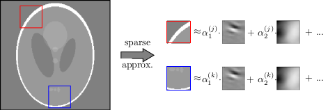
In order to implement this, we first need the analyze function where we can reuse the matchingpursuit function from Wavelets.jl

function analyzeImage(x::Vector{T},D::Matrix{T},xsize::NTuple{2,Int64},
                      psize::NTuple{2,Int64};t0::Int64=size(D,2),tol=1e-3) where T
  nx,ny = xsize
  px,py = psize
  x = reshape(x,nx,ny)
  x_pad = repeat(x,2,2)[1:nx+px-1,1:ny+py-1] # pad image using periodic boundary conditions
  α = zeros(T,size(D,2),nx,ny)
  patch = zeros(T,px*py)
  for j=1:ny
    for i=1:nx
      patch[:] .= vec(x_pad[i:i+px-1,j:j+py-1])
      norm(patch)==0 && continue
      # matchingpursuit is contained in Wavelets.jl
      α[:,i,j] .= matchingpursuit(patch, x->D*x, x->transpose(D)*x, tol)
    end
  end
  return vec(α)
end

Synthetization can be done by

function synthesizeImage(α::Vector{T},D::Matrix{T},xsize::NTuple{2,Int64},psize::NTuple{2,Int64}) where T
  nx,ny = xsize
  px,py = psize
  x = zeros(T,nx+px-1,ny+py-1)
  α = reshape(α,:,nx,ny)
  for j=1:ny
    for i=1:nx
      x[i:i+px-1,j:j+py-1] .+= reshape(D*α[:,i,j],px,py)
    end
  end
  return vec(x[1:nx,1:ny])/(px*py)
end

Once we have those two operations we can setup up a dictionary operator:

function dictOp(D::Matrix{T},xsize::NTuple{2,Int64},psize::NTuple{2,Int64},tol::Float64=1.e-3) where T
  produ = x->analyzeImage(x,D,xsize,psize,tol=tol)
  ctprodu = x->synthesizeImage(x,D,xsize,psize)
  return LinearOperator(prod(xsize)*size(D,2),prod(xsize),false,false
          , produ
          , nothing
          , ctprodu )
end

To test our method, let us load some simulated data and subsample it

# phantom
img = readdlm("data/mribrain100.tsv")

acqData = AcquisitionData(ISMRMRDFile("data/acqDataBrainSim100.h5"))
nx,ny = acqData.encodingSize

# undersample kspace data
acqData = sample_kspace(acqData, 2.0, "poisson", calsize=25,profiles=false);

Now we load a pre-trained dictionary, build the sparsifying transform and perform the reconstruction

# load the dictionary
D = ComplexF64.(readdlm("data/brainDict98.tsv"))

# some parameters
px, py = (6,6)  # patch size
K = px*py       # number of atoms

# CS reconstruction using Wavelets
params = Dict{Symbol,Any}()
params[:reco] = "standard"
params[:reconSize] = (nx,ny)
params[:iterations] = 50
params[:λ] = 2.e-2
params[:regularization] = "L1"
params[:sparseTrafo] = dictOp(D,(nx,ny),(px,py),2.e-2)
params[:ρ] = 0.1
params[:solver] = "admm"
params[:absTol] = 1.e-4
params[:relTol] = 1.e-2

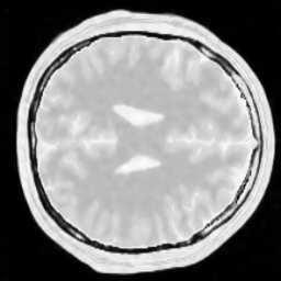
img_d = reconstruction(acqData,params)

For comparison, let us perform the same reconstruction as above but with a Wavelet transform

delete!(params, :sparseTrafo)
params[:sparseTrafoName] = "Wavelet"

img_w = reconstruction(acqData,params)

The following pictures shows the wavelet based CS reconstruction on the left and the dictionary based CS reconstruction on the right:

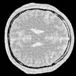
For reference, the original data is shown here:

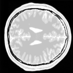
One can clearly see that the dictionary approach performs better than a simple Wavelet L1 prior.