
SymbolicRegression.jl searches for symbolic expressions which optimize a particular objective.
| Latest release | Documentation | Build status | Coverage |
|---|---|---|---|
 |
Check out PySR for a Python frontend.
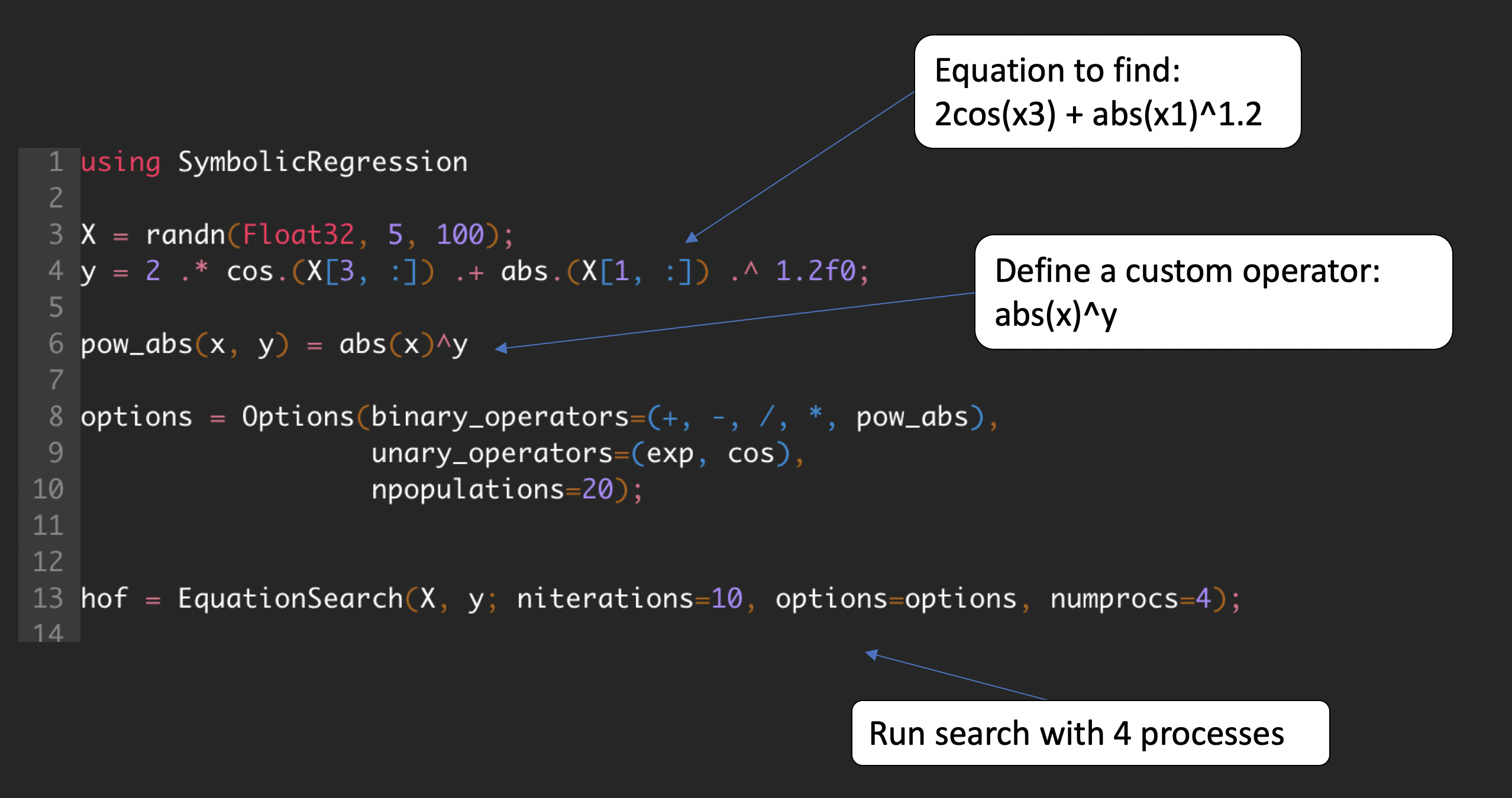
Quickstart
Install in Julia with:
using Pkg
Pkg.add("SymbolicRegression")
The heart of this package is the EquationSearch function, which takes a 2D array (shape [features, rows]) and attempts to model a 1D array (shape [rows]) using analytic functional forms.
Run with:
using SymbolicRegression
X = randn(Float32, 5, 100)
y = 2 * cos.(X[4, :]) + X[1, :] .^ 2 .- 2
options = SymbolicRegression.Options(
binary_operators=[+, *, /, -],
unary_operators=[cos, exp],
npopulations=20
)
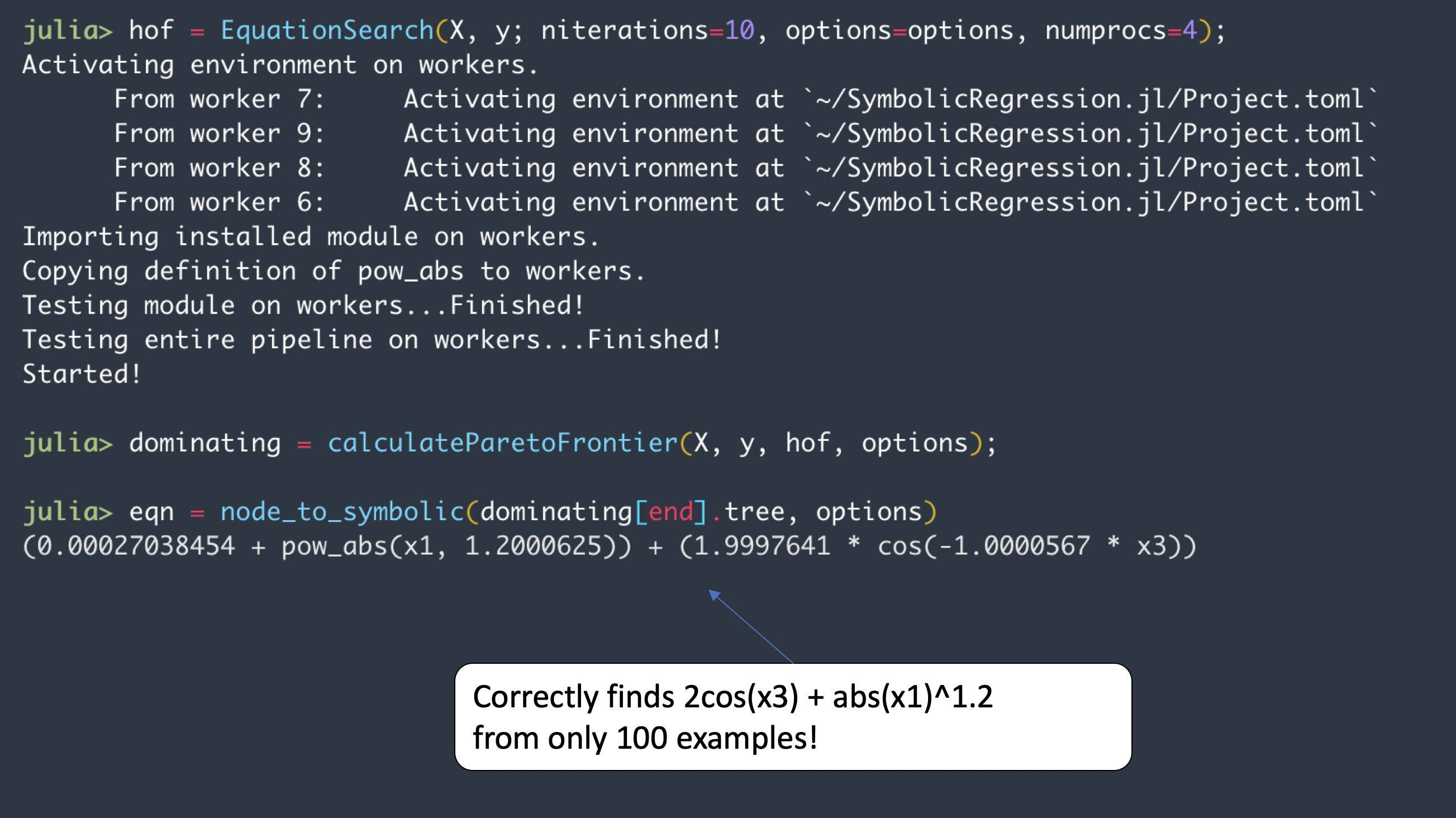
hall_of_fame = EquationSearch(
X, y, niterations=40, options=options,
parallelism=:multithreading
)You can view the resultant equations in the dominating Pareto front (best expression seen at each complexity) with:
dominating = calculate_pareto_frontier(X, y, hall_of_fame, options)This is a vector of PopMember type - which contains the expression along with the score. We can get the expressions with:
trees = [member.tree for member in dominating]Each of these equations is a Node{T} type for some constant type T (like Float32).
You can evaluate a given tree with:
tree = trees[end]
output, did_succeed = eval_tree_array(tree, X, options)
The output array will contain the result of the tree at each of the 100 rows. This did_succeed flag detects whether an evaluation was successful, or whether encountered any NaNs or Infs during calculation (such as, e.g., sqrt(-1)).
Constructing trees
You can also manipulate and construct trees directly. For example:
using SymbolicRegression

options = Options(;
    binary_operators=[+, -, *, ^, /], unary_operators=[cos, exp, sin]
)
x1, x2, x3 = [Node(; feature=i) for i=1:3]
tree = cos(x1 - 3.2 * x2) - x1^3.2
This tree has Float64 constants, so the type of the entire tree will be promoted to Node{Float64}.
We can convert all constants (recursively) to Float32:
float32_tree = convert(Node{Float32}, tree)We can then evaluate this tree on a dataset:
X = rand(Float32, 3, 100)
output, did_succeed = eval_tree_array(tree, X, options)
Exporting to SymbolicUtils.jl
We can view the equations in the dominating Pareto frontier with:
dominating = calculate_pareto_frontier(X, y, hall_of_fame, options)We can convert the best equation to SymbolicUtils.jl with the following function:
eqn = node_to_symbolic(dominating[end].tree, options)
println(simplify(eqn*5 + 3))
We can also print out the full pareto frontier like so:
println("Complexity\tMSE\tEquation")

for member in dominating
    complexity = compute_complexity(member.tree, options)
    loss = member.loss
    string = string_tree(member.tree, options)

    println("$(complexity)\t$(loss)\t$(string)")
end
Code structure
SymbolicRegression.jl is organized roughly as follows. Rounded rectangles indicate objects, and rectangles indicate functions.
(if you can't see this diagram being rendered, try pasting it into mermaid-js.github.io/mermaid-live-editor)
The HallOfFame objects store the expressions with the lowest loss seen at each complexity.
The dependency structure of the code itself is as follows:
Bash command to generate dependency structure from src directory (requires vim-stream):
echo 'stateDiagram-v2'
IFS=$'\n'
for f in *.jl; do
    for line in $(cat $f | grep -e 'import \.\.' -e 'import \.'); do
        echo $(echo $line | vims -s 'dwf:d$' -t '%s/^\.*//g' '%s/Module//g') $(basename "$f" .jl);
    done;
done | vims -l 'f a--> ' | sort
Search options
See https://astroautomata.com/SymbolicRegression.jl/stable/api/#Options