Example: Interaural Time Delay
Stimuli with a delay applied to one ear causes the sound to be perceived as coming from a different direction [1]. These stimuli are commonly used to investigate source localisation algorithms [2].
[1] Grothe, Benedikt, Michael Pecka, and David McAlpine. "Mechanisms of sound localization in mammals." Physiological reviews 90.3 (2010): 983-1012.
[2] Luke, R., & McAlpine, D. (2019, May). A spiking neural network approach to auditory source lateralisation. In ICASSP 2019-2019 IEEE International Conference on Acoustics, Speech and Signal Processing (ICASSP) (pp. 1488-1492). IEEE. Chicago
Realtime Example: Broadband Signal
In this example we apply a 0.5 ms delay to the second channel (right ear). When presented over headphones this causes the sound to be perceived as arriving from the left, as the sound arrives at the left ear first.
using AuditoryStimuli, Unitful, Plots, Pipe, DSP

source = CorrelatedNoiseSource(Float64, 48u"kHz", 2, 0.2, 1)
itd_left = TimeDelay(2, 0.5u"ms", samplerate=48u"kHz")
sink = DummySampleSink(Float64, 48u"kHz", 2)

for frame = 1:100
    @pipe read(source, 1/100u"s") |> modify(itd_left, _) |> write(sink, _)
end

# Validate the audio pipeline output
plot(sink, label=["Left" "Right"])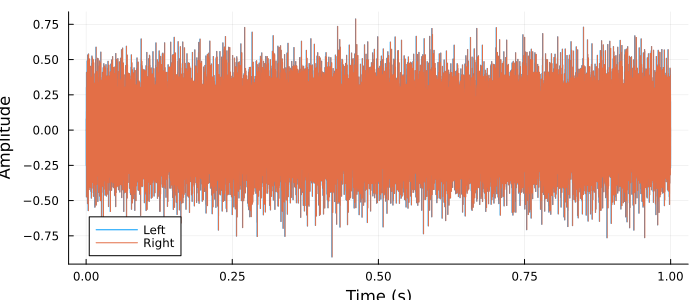
The stimulus output can be validated by observing that the peak in the cross correlation function occurs at 0.5 ms.
plot_cross_correlation(sink, lags=2u"ms")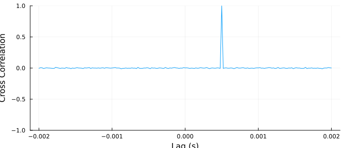
Realtime Example: Narrowband Signal
If we desire a narrowband signal with reduced coherence then we can still use the same functional blocks.
source = CorrelatedNoiseSource(Float64, 48u"kHz", 2, 0.2, 0.6)

responsetype = Bandpass(300, 700; fs=48000)
designmethod = Butterworth(14)
zpg = digitalfilter(responsetype, designmethod)
f_left = DSP.Filters.DF2TFilter(zpg)
f_right = DSP.Filters.DF2TFilter(zpg)
bp = AuditoryStimuli.Filter([f_left, f_right])

itd_left = TimeDelay(2, 1.25u"ms", samplerate=48u"kHz")
sink = DummySampleSink(Float64, 48u"kHz", 2)

for frame = 1:1000
    @pipe read(source, 1/100u"s") |> modify(bp, _) |> modify(itd_left, _) |> write(sink, _)
end

plot(sink, label=["Left" "Right"])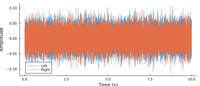
As expected the cross-correlation function will now be damped, but the peak should still be equal to the correlation of the signals, and the peak shift should correspond to the applied time delay.
plot_cross_correlation(sink, lags=4u"ms")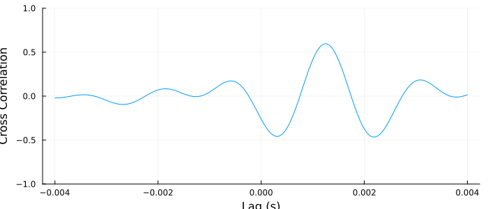
And we can use the convenience function to determine the interaural coherence (IAC) of the signal, which should be approximately 0.6 as set above.
interaural_coherence(sink)0.5959659617941009Whereas if we used the naive correlation implementation from StatsBase we would be extracting the cross correlation value at zero.
using Statistics
cor(sink.buf)[2, 1]-0.261278574635491However, note that if we compute the IAC over a restricted range of lags then we will miss the peak and thus not report the global maximum. By default, as above, the entire range of available lags is used. So if we use only a 1 ms window, whereas the itd was 1.25 ms, the IAC will be under reported.
interaural_coherence(sink, lags=1u"ms")0.4140820136984554