Real-Time Audio Processing
In this tutorial the basics of real-time audio processing are introduced, and how you can generate real time audio with this package.
It is common to process audio in small chunks of samples called frames. This is more efficient than processing signals on a sample by sample basis, yet allows dynamic adaptation of the audio signal. In this example we use a frame size of 1/100th of a second, or 480 samples when using a sample rate of 48 kHz. However, the frame size can be adjusted to suit your research needs.
Real-time processing consists of a source, zero or more modifiers, and a sink. Sources generate the raw signal. Modifiers alter the signal. Sinks are a destination for the signals, typically a sound card, but in this example we use a buffer.
First the required packages are loaded and the sample rate and number of audio channels is specified. This package makes extensive use of units to minimise the chance of coding mistakes, below the sample rate is specified in the unit of kHz.
using AuditoryStimuli, Unitful, Plots, Pipe, DSP

sample_rate = 48u"kHz"
audio_channels = 2
source_rms = 0.2
Set up the signal pipeline components
First we need a source. In this example a simple white noise source is used. The type of data (floats) is specified, as is the the sample rate, number of channels, and the RMS of each channel.
source = NoiseSource(Float64, sample_rate, audio_channels, source_rms)A sink is also required. This would typically be a sound card, but that is not possible with a web page tutorial. Instead, for this website example a dummy sink is used, which simply saves the sample to a buffer. Dummy sink are also useful for validating our generated stimuli, as we can measure and plot the output.
sink = DummySampleSink(Float64, sample_rate, audio_channels)

# But on a real system you would use something like
# devices = PortAudio.devices()
# println(devices)
# sink = PortAudioStream(devices[3], sample_rate, audio_channels)
DummySampleSink{Float64}(48000.0, Matrix{Float64}(undef, 0, 2))In this example a single signal modifier is used. This signal modifier simply adjusts the amplitude of the signal with a linear scaling. We specify the desired linear amplification to be 1.0, so no modification to the amplitude. However, we do not want the signal to jump from silent to full intensity, so we specify the current value of the amplitude as 0 (silent) and set the maximum increase per frame to be 0.05. This will ramp the signal from silent to full intensity.
amp = Amplification(current=0.0, target=1.0, change_limit=0.05)Run the real-time audio pipeline
To run the real-time processing we generate a pipeline and run it. We use the pipe notation to conveniently describe the audio pipeline. In this simple example we read a frame with duration 1/100th of a second from the source. The frame of white noise is piped through the amplitude modifier, and then piped in to the sink. Modifiers always take the modification object as the first argument, followed by an underscore to represent the piped data. Similarly, when writing the data to a sink, the sink is always the first argument, followed by an underscore to represent the piped data. The pipeline is run 100 times, resulting in 1 second of generated audio.
for frame = 1:100
    @pipe read(source, 0.01u"s") |> modify(amp, _) |> write(sink, _)
end
Verify processing was correctly applied
We can plot the data from sink (as it was a DummySink, which is simply a buffer) to confirm the signal generated matches our expectations. As expected, we see below that two channels of audio are generated, that the signal is 1 second long, and that there is a ramp applied to the onset.
plot(sink)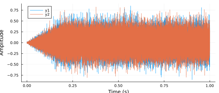
Apply a filter modifier
A more advanced application is to use a filter as a modifier. The filter maintains its state between calls, so can be used for real-time audio processing. Below a bandpass filter is designed, for more details on filter design using the DSP package see this documentation.
responsetype = Bandpass(500, 4000; fs=48000)
designmethod = Butterworth(4)
zpg = digitalfilter(responsetype, designmethod)
Once the filter is specified as a zero pole gain representation two filters are instantiated using this specification. A filter must be generated for each channel of audio. These DSP.Filters are then passed in to the AuditoryStimuli filter object for further use.
f_left = DSP.Filters.DF2TFilter(zpg)
f_right = DSP.Filters.DF2TFilter(zpg)
bandpass = AuditoryStimuli.Filter([f_left, f_right])
Once the filters are designed and placed in an AuditoryStimuli.Filter object they can be used just like any other modifier. Below the filter is included in the pipeline and applied to 1 second of audio in 1/100th second frames. This example demonstrates how an arbitrary number of modifiers can be chained to create complex audio stimuli.
for frame = 1:100
    @pipe read(source, 0.01u"s") |> modify(amp, _) |> modify(bandpass, _) |> write(sink, _)
end
Modifying modifier parameters
Further, the parameters of modifiers can be varied at any time. This can be handy to adapt your stimuli to user responses or feedback. Below the target amplification is updated to be set to zero. This effectively ramps off the signal.
setproperty!(amp, :target, 0.0)
for frame = 1:20
    @pipe read(source, 0.01u"s") |> modify(amp, _) |> modify(bandpass, _) |> write(sink, _)
end
Verify output
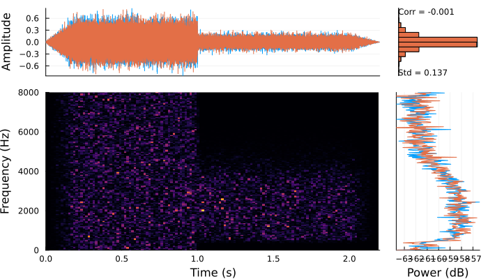
The entire signal (both the amplification, then the filtering sections) can be viewed using the convenience plotting function below. We observe that the signal is ramped on due to the amplification modifier. We can then see that at 1 second the spectral content of the signal was modified. And finally the signal is ramped off.
PlotSpectroTemporal(sink, figure_size=(700, 400), frequency_limits = [0, 8000])