A freezing bucket

A common laboratory experiment freezes an insultated bucket of water from the top down, using a metal lid to keep the top of the bucket at some constant, very cold temperature. In this example, we simulate such a scenario using SlabSeaIceModel. Here, the bucket is perfectly insulated and infinitely deep, like many buckets are: if the Simulation is run for longer, the ice will keep freezing, and freezing, and will never run out of water. Also, the water in the infinite bucket is (somehow) all at the same temperature, in equilibrium with the ice-water interface (and therefore fixed at the melting temperature). Yep, this kind of thing happens all the time.

We start by using Oceananigans to bring in functions for building grids and Simulations and the like.

using Oceananigans
using Oceananigans.Units

Next we using ClimaSeaIce to get some ice-specific names.

using ClimaSeaIce

An infinitely deep bucket with a single grid point

Perhaps surprisingly, we need just one grid point to model an possibly infinitely thick slab of ice with SlabSeaIceModel. We would only need more than 1 grid point if our boundary conditions vary in the horizontal direction.

grid = RectilinearGrid(size=(), topology=(Flat, Flat, Flat))

1×1×1 RectilinearGrid{Float64, Oceananigans.Grids.Flat, Oceananigans.Grids.Flat, Oceananigans.Grids.Flat} on Oceananigans.Architectures.CPU with 0×0×0 halo
├── Flat x
├── Flat y
└── Flat z

Next, we build our model of an ice slab freezing into a bucket. We start by defining a constant internal ConductiveFlux with ice_conductivity

conductivity = 2 # kg m s⁻³ K⁻¹
internal_heat_flux = ConductiveFlux(; conductivity)

ConductiveFlux{Float64}(2.0)

Note that other units besides Celsius can be used, but that requires setting model.phase_transitions` with appropriate parameters. We set the ice heat capacity and density as well,

ice_heat_capacity = 2100 # J kg⁻¹ K⁻¹
ice_density = 900 # kg m⁻³
phase_transitions = PhaseTransitions(; ice_heat_capacity, ice_density)

PhaseTransitions{Float64, ClimaSeaIce.LinearLiquidus{Float64}}(900.0, 2100.0, 999.8, 4186.0, 334000.0, 0.0, ClimaSeaIce.LinearLiquidus{Float64}(0.0, 0.054))

We set the top ice temperature,

top_temperature = -10 # ᵒC
top_heat_boundary_condition = PrescribedTemperature(-10)

PrescribedTemperature{Int64}(-10)

Then we assemble it all into a model,

model = SlabSeaIceModel(grid;
                        internal_heat_flux,
                        phase_transitions,
                        top_heat_boundary_condition)

SlabSeaIceModel{Oceananigans.Architectures.CPU, Oceananigans.Grids.RectilinearGrid}(time = 0 seconds, iteration = 0)
├── grid: 1×1×1 RectilinearGrid{Float64, Oceananigans.Grids.Flat, Oceananigans.Grids.Flat, Oceananigans.Grids.Flat} on Oceananigans.Architectures.CPU with 0×0×0 halo
├── top_surface_temperature: ConstantField(-10)
├── minimium_ice_thickness: ConstantField(0.0)
└── external_heat_fluxes: 
    ├── top: FluxFunction of slab_internal_heat_flux with parameters (flux=ConductiveFlux{Float64}, liquidus=ClimaSeaIce.LinearLiquidus{Float64}, bottom_heat_boundary_condition=ClimaSeaIce.HeatBoundaryConditions.IceWaterThermalEquilibrium{Int64})
    └── bottom: 0

Note that the default bottom heat boundary condition for SlabSeaIceModel is IceWaterThermalEquilibrium with freshwater. That's what we want!

model.heat_boundary_conditions.bottom

ClimaSeaIce.HeatBoundaryConditions.IceWaterThermalEquilibrium{Int64}(0)

Ok, we're ready to freeze the bucket for 10 straight days with an initial ice thickness of 1 cm,

simulation = Simulation(model, Δt=10minute, stop_time=10days)

set!(model, h=0.01)

Collecting data and running the simulation

Before simulating the freezing bucket, we set up a Callback to create a timeseries of the ice thickness saved at every time step.

# Container to hold the data
timeseries = []

# Callback function to collect the data from the `sim`ulation
function accumulate_timeseries(sim)
    h = sim.model.ice_thickness
    push!(timeseries, (time(sim), first(h)))
end

# Add the callback to `simulation`
simulation.callbacks[:save] = Callback(accumulate_timeseries)

Callback of accumulate_timeseries on IterationInterval(1)

Now we're ready to hit the Big Red Button (it should run pretty quick):

run!(simulation)

[ Info: Initializing simulation...
[ Info:     ... simulation initialization complete (218.453 ms)
[ Info: Executing initial time step...
[ Info:     ... initial time step complete (229.360 ms).
[ Info: Simulation is stopping after running for 621.364 ms.
[ Info: Simulation time 10 days equals or exceeds stop time 10 days.

Visualizing the result

It'd be a shame to run such a "cool" simulation without looking at the results. We'll visualize it with Makie.

using CairoMakie

timeseries is a Vector of Tuple. So we have to do a bit of processing to build Vectors of time t and thickness h. It's not much work though:

t = [datum[1] for datum in timeseries]
h = [datum[2] for datum in timeseries]

1441-element Vector{Float64}:
 0.01
 0.01359353307787306
 0.01623709384848865
 0.018450256568002983
 0.02039794388857124
 0.02215965727375536
 0.023781312804560452
 0.025292387112108326
 0.026713183441827916
 0.028058411757913317
 ⋮
 0.32116543894477484
 0.32127732934897524
 0.3213891807854011
 0.3215009932947423
 0.32161276691761814
 0.3217245016945772
 0.3218361976660977
 0.32194785487258765
 0.3220594733543848

Just for fun, we also compute the velocity of the ice-water interface:

dhdt = @. (h[2:end] - h[1:end-1]) / simulation.Δt

1440-element Vector{Float64}:
 5.9892217964551e-6
 4.405934617692647e-6
 3.6886045325238912e-6
 3.2461455342804267e-6
 2.9361889753068706e-6
 2.702759218008484e-6
 2.5184571792464564e-6
 2.367993882865984e-6
 2.242047193475669e-6
 2.134554816619639e-6
 ⋮
 1.8654902122651936e-7
 1.864840070006646e-7
 1.8641906070972676e-7
 1.8635418223537463e-7
 1.862893714597395e-7
 1.862246282651377e-7
 1.861599525341632e-7
 1.860953441498725e-7
 1.8603080299522957e-7

All that's left, really, is to put those lines! in an Axis:

set_theme!(Theme(fontsize=24, linewidth=4))

fig = Figure(size=(1200, 600))

axh = Axis(fig[1, 1], xlabel="Time (days)", ylabel="Ice thickness (cm)")
axd = Axis(fig[1, 2], xlabel="Ice thickness (cm)", ylabel="Freezing rate (μm s⁻¹)")

lines!(axh, t ./ day, 1e2 .* h)
lines!(axd, 1e2 .* h[1:end-1], 1e6 .* dhdt)

fig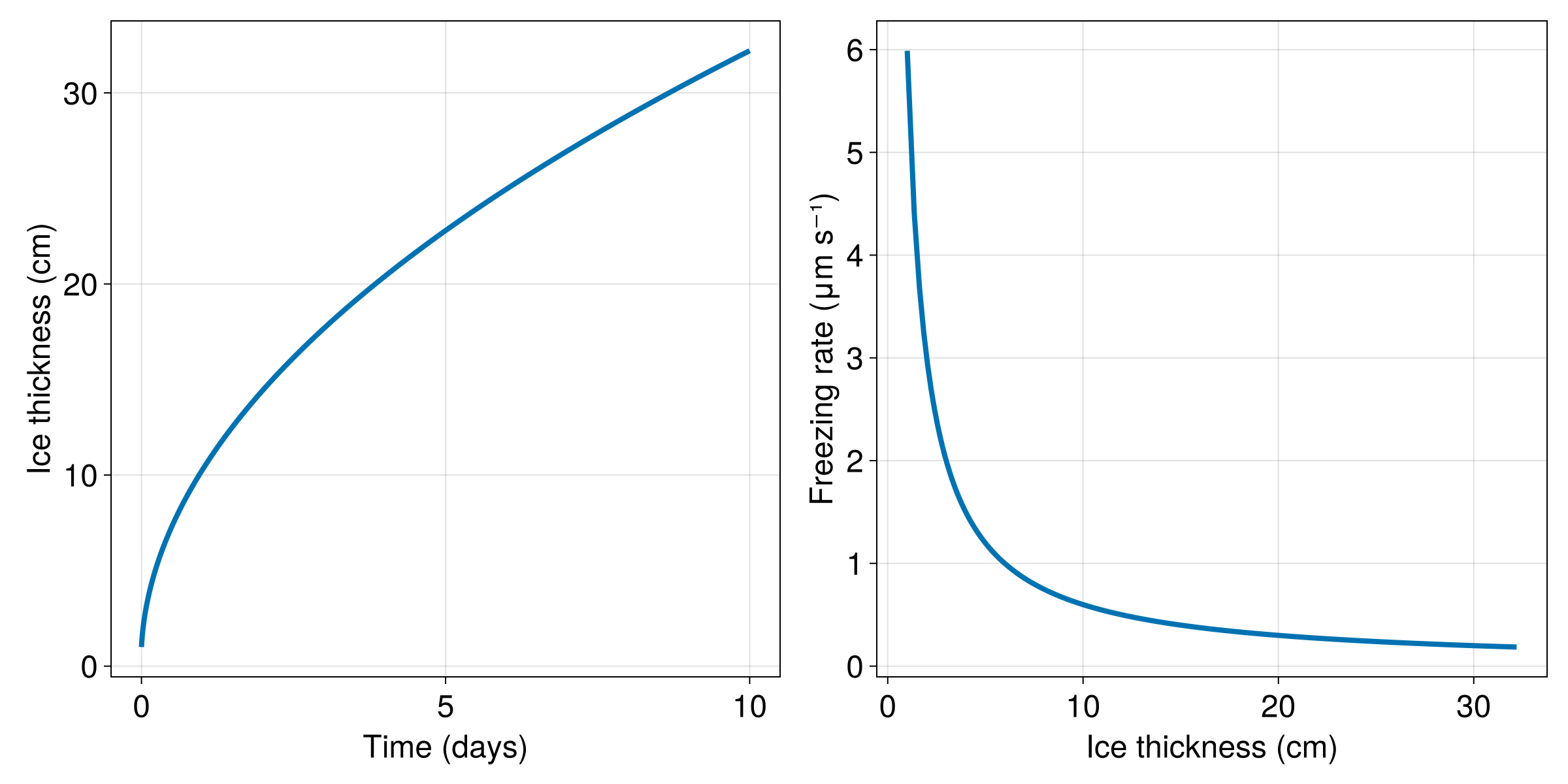

If you want more ice, you can increase simulation.stop_time and run!(simulation) again (or just re-run the whole script).

This page was generated using Literate.jl.