Atomic and group contributions

One of the interesting features of Minimum-Distance distributions is that they can be naturally decomposed into the atomic or group contributions. Simply put, if a MDDF has a peak at a hydrogen-bonding distance, it is natural to decompose that peak into the contributions of each type of solute or solvent atom to that peak.

To obtain the atomic contributions of an atom or group of atoms to the MDDF, the coordination number, or the site count at each distance, the contributions function is provided. For example, in a system composed of a protein and water, we would have defined the solute and solvent using:

using PDBTools, ComplexMixtures
atoms = readPDB("system.pdb")
protein = select(atoms,"protein")
water = select(atoms,"water")
solute = AtomSelection(protein,nmols=1)
solvent = AtomSelection(water,natomspermol=3)

The MDDF calculation is executed with:

trajectory = Trajectory("trajectory.dcd",solute,solvent)
results = mddf(trajectory, Options(bulk_range=(8.0, 12.0)))

Atomic contributions in the result data structure

The results data structure contains the decomposition of the MDDF into the contributions of every type of atom of the solute and the solvent. These contributions can be retrieved using the contributions function, with the SoluteGroup and SolventGroup selectors.

For example, if the MDDF of water (solvent) relative to a solute was computed, and water has atom names OH2, H1, H2, one can retrieve the contributions of the oxygen atom with:

OH2 = contributions(results, SolventGroup(["OH2"]))

or with, if OH2 is the first atom in the molecule,

OH2 = contributions(results, SolventGroup([1]))

The contributions of the hydrogen atoms can be obtained, similarly, with:

H = contributions(results, SolventGroup(["H1", "H2"]))

or with, if OH2 is the first atom in the molecule,

H = contributions(results, SolventGroup([2, 3]))

Each of these calls will return a vector of the constributions of these atoms to the total MDDF.

For example, here we plot the total MDDF and the Oxygen contributions:

using Plots
plot(results.d, results.mddf, label=["Total MDDF"], linewidth=2)
plot!(results.d, contributions(results, SolventGroup(["OH2"])), label=["OH2"], linewidth=2)
plot!(xlabel="Distance / Å", ylabel="MDDF")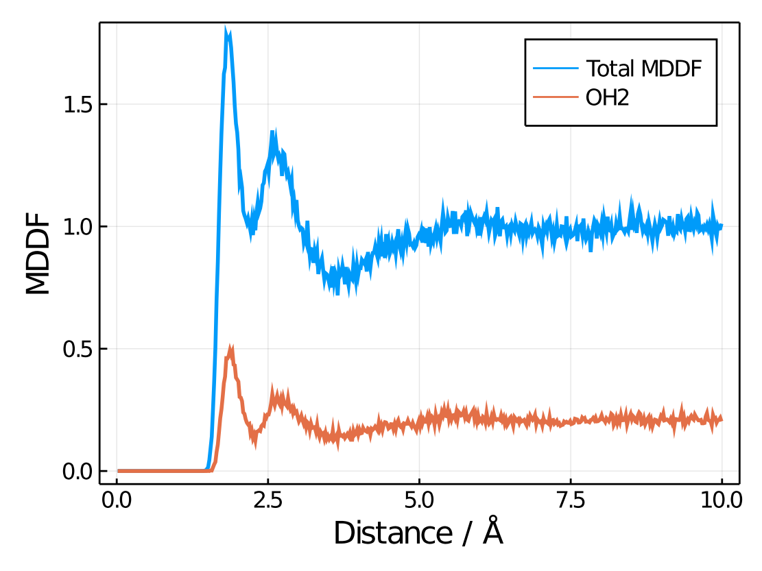

Contributions to coordination numbers or site counts

The keyword type defines the return type of the contribution:

type=:mddf : the contribution of the group to the MDDF is returned (default).
type=:coordination_number : the contribution of the group to the coordination number, that is, the cumulative sum of counts at each distance, is returned.
type=:md_count : the contribution of the group to the site count at each distance is returned.

Example of the usage of the type option:

ca_contributions = contributions(results, SoluteGroup(["CA"]); type=:coordination_number)

Using PDBTools

If the solute is a protein, or other complex molecule, selections defined with PDBTools can be used. For example, this will retrieve the contribution of the acidic residues of a protein to total MDDF:

using PDBTools
atoms = readPDB("system.pdb")
acidic_residues = select(atoms, "acidic")
acidic_contributions = contributions(results, SoluteGroup(acidic_residues))

It is expected that for a protein most of the atoms do not contribute to the MDDF, and that all values are zero at very short distances, smaller than the radii of the atoms.

More interesting and general is to select atoms of a complex molecule, like a protein, using residue names, types, etc. Here we illustrate how this is done by providing selection strings to contributions to obtain the contributions to the MDDF of different types of residues of a protein to the total MDDF.

For example, if we want to split the contributions of the charged and neutral residues to the total MDDF distribution, we could use to following code. Here, solute refers to the protein.

charged_residues = PDBTools.select(atoms,"charged")
charged_contributions = contributions(results, SoluteGroup(charged_residues))

neutral_residues = PDBTools.select(atoms,"neutral")
neutral_contributions = contributions(atoms, SoluteGroup(neutral_residues))

The charged_contributions and neutral_contributions outputs are vectors containing the contributions of these residues to the total MDDF. The corresponding plot is:

plot(results.d,results.mddf,label="Total MDDF",linewidth=2)
plot!(results.d,charged_contributions,label="Charged residues",linewidth=2)
plot!(results.d,neutral_contributions,label="Neutral residues",linewidth=2)
plot!(xlabel="Distance / Å",ylabel="MDDF")

Resulting in:

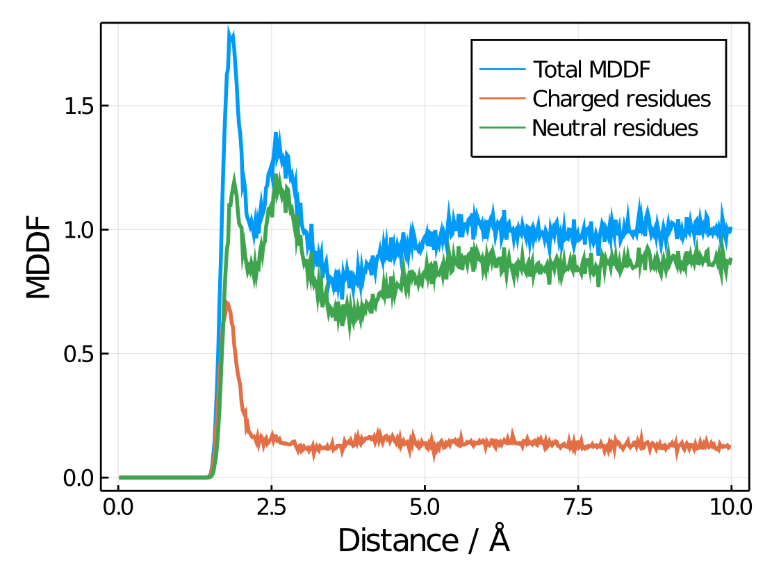
Note here how charged residues contribute strongly to the peak at hydrogen-bonding distances, but much less in general. Of course all selection options could be used, to obtain the contributions of specific types of residues, atoms, the backbone, the side-chains, etc.

Reference functions

ComplexMixtures.ResidueContributions — Type

ResidueContributions (data structure)

Constructor function:

ResidueContributions(
    results::Result, atoms::AbstractVector{PDBTools.Atom};
    dmin=1.5, dmax=3.5,
    type=:mddf,
)

Compute the residue contributions to the solute-solvent pair distribution function. The function returns a ResidueContributions object that can be used to plot the residue contributions, or to perform arithmetic operations with other ResidueContributions objects.

Arguments

results::Result: The result object obtained from the mddf function.
atoms::AbstractVector{PDBTools.Atom}: The vector of atoms of the solute, or a part of it.

Optional arguments

dmin::Float64: The minimum distance to consider. Default is 1.5.
dmax::Float64: The maximum distance to consider. Default is 3.5.
type::Symbol: The type of the pair distribution function (:mddf, :md_count, or :coordination_number). Default is :mddf.
silent::Bool: If true, the progress bar is not shown. Default is false.

A structure of type ResultContributions can be used to plot the residue contributions to the solute-solvent pair distribution function, using the Plots.contourf function, and to perform arithmetic operations with other ResidueContributions objects, multiplying or dividing by a scalar, and slicing (see examples below).

Examples

Constructing a ResidueContributions object

julia> using ComplexMixtures, PDBTools

julia> using ComplexMixtures.Testing: data_dir; ComplexMixtures._testing_show_method[] = true; # testing mode

julia> atoms = readPDB(data_dir*"/NAMD/Protein_in_Glycerol/system.pdb");

julia> results = load(data_dir*"/NAMD/Protein_in_Glycerol/protein_glyc.json");

julia> rc = ResidueContributions(results, select(atoms, "protein"); silent=true)

          Residue Contributions
     3.51 █     █      █     █            █
     3.27 █              █   █
     3.03 █     █    █       █            █       █       █                █
     2.79 █    ██    █ █ █   █            █      ██          █        █    █
 d   2.55 █ █  ██    █ █ █   █            ██     ██ █  █  █  █  █     █    █
     2.31 █ █  ██    █ ███   █    ██      ██     ██ █  ██ █  ██ █     █    █
     2.07 █ █   █  █ █████   █    ██      ██     ██ █  ██ █  █ ██    █     █
     1.83 █   █ █  █ █████   █    ██      █      ██ █  ██    █ ██     █    █
     1.59
         A1      T33     T66     S98     S130    T162    A194    H226    G258

Plotting

using ComplexMixtures, PDBTools, Plots
...
result = mddf(traj, options)
rc = ResidueContributions(result, select(atoms, "protein"))
contourf(rc) # plots a contour map

Slicing

Slicing, or indexing, the residue contributions returns a new ResidueContributions object with the selected residues:

using ComplexMixtures, PDBTools, Plots
...
result = mddf(traj, options)
rc = ResidueContributions(result, select(atoms, "protein"))
rc_7 = rc[7] # contributions of residue 7
rc_range = rc[10:50] # slice the residue contributions
contourf(rc_range) # plots a contour map of the selected residues

Arithmetic operations

using ComplexMixtures, PDBTools, Plots
...
# first simulation (for example, low temperature):
result1 = mddf(traj2, options)
rc1 = ResidueContributions(result1, select(atoms, "protein"))
# second simulation (for example, high temperature):
result2 = mddf(traj2, options)
rc2 = ResidueContributions(result2, select(atoms, "protein"))
# difference of the residue contributions between the two simulations:
rc_diff = rc2 - rc1
contourf(rc_diff) # plots a contour map of the difference

Compat

Slicing, indexing, and multiplication and divison by scalars were introduces in v2.7.0.

ComplexMixtures.contributions — Method

contributions(R::Result, group::Union{SoluteGroup,SolventGroup}; type = :mddf)

Returns the contributions of the atoms of the solute or solvent to the MDDF, coordination number, or MD count.

Arguments

R::Result: The result of a calculation.
group::Union{SoluteGroup,SolventGroup}: The group of atoms to consider.
type::Symbol: The type of contributions to return. Can be :mddf (default), :coordination_number, or :md_count.

Examples

julia> using ComplexMixtures, PDBTools

julia> dir = ComplexMixtures.Testing.data_dir*"/Gromacs";

julia> atoms = readPDB(dir*"/system.pdb");

julia> protein = select(atoms, "protein");

julia> emim = select(atoms, "resname EMI"); 

julia> solute = AtomSelection(protein, nmols = 1)
AtomSelection 
    1231 atoms belonging to 1 molecule(s).
    Atoms per molecule: 1231
    Number of groups: 1231

julia> solvent = AtomSelection(emim, natomspermol = 20)
AtomSelection 
    5080 atoms belonging to 254 molecule(s).
    Atoms per molecule: 20
    Number of groups: 20

julia> results = load(dir*"/protein_EMI.json"); # load pre-calculated results

julia> ca_cb = contributions(results, SoluteGroup(["CA", "CB"])); # contribution of CA and CB atoms to the MDDF

julia> ca_cb = contributions(results, SoluteGroup(["CA", "CB"]); type=:coordination_number); # contribution of CA and CB atoms to the coordination number