Tools

Coordination numbers
2D density map per residue
3D density map around a macromolecule
Overview of the solvent and solute properties
Computing radial distribution functions

Coordination numbers

The function

coordination_number(R::Result, group::Union{SoluteGroup, SolventGroup})

computes the coordination number of a given group of atoms from the solute or solvent atomic contributions to the MDDF. Here, R is the result of the mddf calculation, and group_contributions is the output of the contributions function for the desired set of atoms.

If no group is defined, the coordination number of the complete solute is returned, which is equivalent to the R.coordination_number field of the Result data structure:

coordination_number(R::Result) == R.coordination_number

Note

There are some systems for which the normalization of the distributions is not necessary or possible. It is still possible to compute the coordination numbers, by running, instead of mddf, the coordination_number function:

coordination_number(trajectory::Trajectory, options::Options)

This call will return Result data structure but with all fields requiring normalization with zeros. In summary, this result data structure can be used to compute the coordination numbers, but not the MDDF, RDF, or KB integrals.

Compat

The independent computation of coordination numbers was introduced in version 1.1.

Example

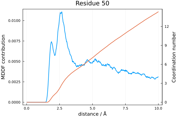
In the following example we compute the coordination number of the atoms of residue 50 (which belongs to the solute - a protein) with the solvent atoms of TMAO, as a function of the distance. The plot produced will show side by side the residue contribution to the MDDF and the corresponding coordination number.

using ComplexMixtures, PDBTools
using Plots, EasyFit
pdb = readPDB("test/data/NAMD/structure.pdb")
R = load("test/data/NAMD/protein_tmao.json")
solute = AtomSelection(PDBTools.select(pdb, "protein"), nmols=1)
residue50 = PDBTools.select(pdb, "residue 50")
# Compute the group contribution to the MDDF
residue50_contribution = contributions(R, SoluteGroup(residue50))
# Now compute the coordination number
residue50_coordination = coordination_number(R, SoluteGroup(residue50))
# Plot with twin y-axis
plot(R.d, movavg(residue50_contribution,n=10).x,
    xaxis="distance / Å", 
    yaxis="MDDF contribution", 
    linewidth=2, label=nothing, color=1
)
plot!(twinx(),R.d, residue50_coordination, 
    yaxis="Coordination number", 
    linewidth=2, label=nothing, color=2
)
plot!(title="Residue 50", framestyle=:box, subplot=1)

With appropriate input data, this code produces:

ComplexMixtures.coordination_number — Function

coordination_number(R::Result) = R.coordination_number
coordination_number(R::Result, s::Union{SoluteGroup,SolventGroup})

Computes the coordination number of a given group of atoms of the solute or solvent

atomic contributions to the MDDF. If no group is defined (first call above), the coordination number of the whole solute or solvent is returned.

If the group_contributions to the mddf are computed previously with the contributions function, the result can be used to compute the coordination number by calling coordination_number(R::Result, group_contributions).

Otherwise, the coordination number can be computed directly with the second call, where:

s is the solute or solvent selection (type ComplexMixtures.AtomSelection)

atom_contributions is the R.solute_atom or R.solvent_atom arrays of the Result structure

R is the Result structure,

and the last argument is the selection of atoms from the solute to be considered, given as a list of indices, list of atom names, or a selection following the syntax of PDBTools, or vector of PDBTools.Atoms, or a PDBTools.Residue

Examples

In the following example we compute the coordination number of the atoms of residue 50 (of the solute) with the solvent atoms of TMAO, as a function of the distance. Finally, we show the average number of TMAO molecules within 5 Angstroms of residue 50. The findlast(<(5), R.d) part of the code below returns the index of the last element of the R.d array that is smaller than 5 Angstroms.

Precomputing the group contributions Using the contributions function

using ComplexMixtures, PDBTools
pdb = readPDB("test/data/NAMD/structure.pdb");
R = load("test/data/NAMD/protein_tmao.json");
solute = AtomSelection(PDBTools.select(pdb, "protein"), nmols=1);
residue50 = PDBTools.select(pdb, "residue 50");
# Compute the group contributions to the MDDF
residue50_contribution = contributions(solute, R.solute_atom, residue50);
# Now compute the coordination number
residue50_coordination = coordination_number(R, residue50_contribution)
# Output the average number of TMAO molecules within 5 Angstroms of residue 50
residue50_coordination[findlast(<(5), R.d)]

Without precomputing the group_contribution

using ComplexMixtures, PDBTools
pdb = readPDB("test/data/NAMD/structure.pdb");
R = load("test/data/NAMD/protein_tmao.json");
solute = AtomSelection(PDBTools.select(pdb, "protein"), nmols=1);
residue50 = PDBTools.select(pdb, "residue 50");
# Compute the coordination number
residue50_coordination = coordination_number(solute, R.solute_atom, R, group)
# Output the average number of TMAO molecules within 5 Angstroms of residue 50
residue50_coordination[findlast(<(5), R.d)]

2D density map per residue

One nice way to visualize the accumulation or depletion of a solvent around a macromolecule (a protein, for example), is to obtain a 2D map of the density as a function of the distance from its surface. For example, in the figure below the density of a solute (here, Glycerol), in the neighborhood of a protein is shown:

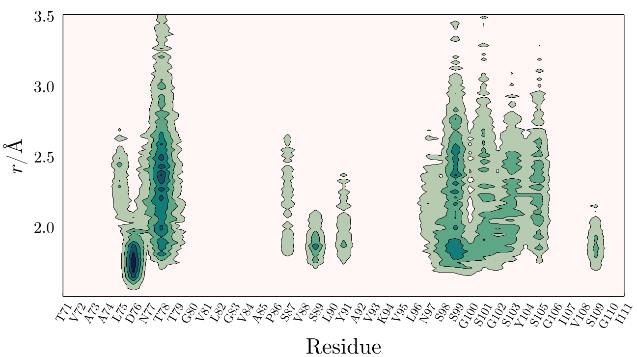
Here, one can see that Glycerol accumulates on Asp76 and on the proximity of hydrogen-bonding residues (Serine residues mostly). This figure was obtained by extracting from atomic contributions of the protein the contribution of each residue to the MDDF, coordination numbers or minimum-distance counts.

Compat

All features described in this section are only available in v2.7.0 or greater.

The computation of the contributions of each residue can be performed with the convenience function ResidueContributions, which creates an object containing the contributions of the residues to the mddf (or coordination numbers, or minimum-distance counts), the residue names, and distances:

ComplexMixtures.ResidueContributions — Type

ResidueContributions (data structure)

Constructor function:

ResidueContributions(
    results::Result, atoms::AbstractVector{PDBTools.Atom};
    dmin=1.5, dmax=3.5,
    type=:mddf,
)

Compute the residue contributions to the solute-solvent pair distribution function. The function returns a ResidueContributions object that can be used to plot the residue contributions, or to perform arithmetic operations with other ResidueContributions objects.

Arguments

results::Result: The result object obtained from the mddf function.
atoms::AbstractVector{PDBTools.Atom}: The vector of atoms of the solute, or a part of it.

Optional arguments

dmin::Float64: The minimum distance to consider. Default is 1.5.
dmax::Float64: The maximum distance to consider. Default is 3.5.
type::Symbol: The type of the pair distribution function (:mddf, :md_count, or :coordination_number). Default is :mddf.
silent::Bool: If true, the progress bar is not shown. Default is false.

A structure of type ResultContributions can be used to plot the residue contributions to the solute-solvent pair distribution function, using the Plots.contourf function, and to perform arithmetic operations with other ResidueContributions objects, multiplying or dividing by a scalar, and slicing (see examples below).

Examples

Constructing a ResidueContributions object

julia> using ComplexMixtures, PDBTools

julia> using ComplexMixtures.Testing: data_dir; ComplexMixtures._testing_show_method[] = true; # testing mode

julia> atoms = readPDB(data_dir*"/NAMD/Protein_in_Glycerol/system.pdb");

julia> results = load(data_dir*"/NAMD/Protein_in_Glycerol/protein_glyc.json");

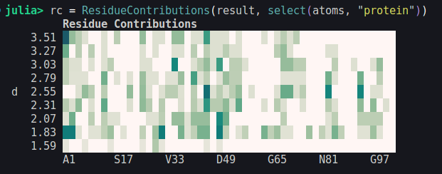
julia> rc = ResidueContributions(results, select(atoms, "protein"); silent=true)

          Residue Contributions
     3.51 █     █      █     █            █
     3.27 █              █   █
     3.03 █     █    █       █            █       █       █                █
     2.79 █    ██    █ █ █   █            █      ██          █        █    █
 d   2.55 █ █  ██    █ █ █   █            ██     ██ █  █  █  █  █     █    █
     2.31 █ █  ██    █ ███   █    ██      ██     ██ █  ██ █  ██ █     █    █
     2.07 █ █   █  █ █████   █    ██      ██     ██ █  ██ █  █ ██    █     █
     1.83 █   █ █  █ █████   █    ██      █      ██ █  ██    █ ██     █    █
     1.59
         A1      T33     T66     S98     S130    T162    A194    H226    G258

Plotting

using ComplexMixtures, PDBTools, Plots
...
result = mddf(traj, options)
rc = ResidueContributions(result, select(atoms, "protein"))
contourf(rc) # plots a contour map

Slicing

Slicing, or indexing, the residue contributions returns a new ResidueContributions object with the selected residues:

using ComplexMixtures, PDBTools, Plots
...
result = mddf(traj, options)
rc = ResidueContributions(result, select(atoms, "protein"))
rc_7 = rc[7] # contributions of residue 7
rc_range = rc[10:50] # slice the residue contributions
contourf(rc_range) # plots a contour map of the selected residues

Arithmetic operations

using ComplexMixtures, PDBTools, Plots
...
# first simulation (for example, low temperature):
result1 = mddf(traj2, options)
rc1 = ResidueContributions(result1, select(atoms, "protein"))
# second simulation (for example, high temperature):
result2 = mddf(traj2, options)
rc2 = ResidueContributions(result2, select(atoms, "protein"))
# difference of the residue contributions between the two simulations:
rc_diff = rc2 - rc1
contourf(rc_diff) # plots a contour map of the difference

Compat

Slicing, indexing, and multiplication and divison by scalars were introduces in v2.7.0.

The output of ResidueContributions is by default shown as a simple unicode plot:

The ResidueContribution object can be used to produce a high-quality contour plot using the Plots.contourf function:

Plots.contourf — Method

contourf(
    rc::ResidueContributions; 
    step::Int=1,
    oneletter=false,
    xlabel="Residue",
    ylabel="r / Å",
)

Plot the contribution of each residue to the solute-solvent pair distribution function as a contour plot. This function requires loading the Plots package.

Arguments

rc::ResidueContributions: The residue contributions to the solute-solvent pair distribution function, as computed by the ResidueContributions function.

Optional arguments

step: The step of the residue ticks in the x-axis of the plot. Default is 1.
oneletter::Bool: Use one-letter residue codes. Default is false. One-letter codes are only available for the 20 standard amino acids.
xlabel and ylabel: Labels for the x and y axes. Default is "Residue" and "r / Å".

This function will set color limits and choose the scale automatically. These parameters can be set with the clims and color arguments of Plots.contourf. Other plot customizations can be done by passing other keyword arguments to this function, which will be passed to Plots.contourf.

Example

julia> using ComplexMixtures, Plots, PDBTools

julia> results = load("mddf.json")

julia> atoms = readPDB("system.pdb", "protein")

julia> rc = ResidueContributions(results, atoms; oneletter=true)

julia> plt = contourf(rc; step=5)

This will produce a plot with the contribution of each residue to the solute-solvent pair distribution function, as a contour plot, with the residues in the x-axis and the distance in the y-axis.

To customize the plot, use the Plot.contourf keyword parameters, for example:

julia> plt = contourf(rc; step=5, size=(800,400), title="Title", clims=(-0.1, 0.1))

Compat

This function requires loading the Plots package and is available in ComplexMixtures v2.5.0 or greater.

Support for all Plots.contourf parameters was introduced in ComplexMixtures v2.6.0.

A complete example of its usage can be seen here.

The ResidueContributions object can be indexes and sliced, for the analysis of the contributions of specific residues or range of residues:

rc = ResidueContributions(results1, select(atoms, "protein")); 
rc_7 = rc[7] # contributions of residue 7
rc_range = rc[20:50] # contributions of a range of residues

Slicing will return a new ResidueContributions object.

Additionally, these ResidueContributions objects can be subtracted, divided, summed, or multiplied, to compare contributions of residues among different simulations. Typically, if one wants to compare the solvation of residues in two different simulations, one can do:

# first simulation (for example, low temperature)
rc1 = ResidueContributions(results1, select(atoms, "protein")); 

# second simulation (for example, high temperature)
rc2 = ResidueContributions(results2, select(atoms, "protein"));

# difference in residue contributions to solvation
rc_diff = rc2 - rc1

# Plot difference
using Plots
contourf(rc_diff; title="Density difference", step=2, colorbar=:left)

Which will produce a plot similar to the one below (the data of this plot is just illustrative):

which will return a new ResidueContributions object.

Finally, it is also possible to renormalize the contributions by multiplication or division by scalars,

rc2 = rc / 15
rc2 = 2 * rc

Tip

This function is a convenience function only.

Basically, we are extracting the contribution of each residue independently and building a matrix where each row represents a distance and each column a residue. Using PDBTools, this can be done with, for example:

residues = collect(eachresidue(protein))
residue_contributions = zeros(length(R.d),length(residues))
for (i,residue) in pairs(residues)
  c = contributions(results, SoluteGroup(residue)) 
  residue_contributions[:,i] .= c
end

The above produces a matrix with a number of columns equal to the number of residues and a number of rows equal to the number of MDDF points. That matrix can be plotted as a contour map with adequate plotting software.

3D density map around a macromolecule

Three-dimensional representations of the distribution functions can also be obtained from the MDDF results. These 3D representations are obtained from the fact that the MDDFs can be decomposed into the contributions of each solute atom, and that each point in space is closest to a single solute atom as well. Thus, each point in space can be associated to one solute atom, and the contribution of that atom to the MDDF at the corresponding distance can be obtained.

A 3D density map is constructed with the grid3D function:

ComplexMixtures.grid3D — Function

grid3D(
    result::Result, atoms, output_file::Union{Nothing,String} = nothing; 
    dmin=1.5, ddax=5.0, step=0.5, silent = false,
)

This function builds the grid of the 3D density function and fills an array of mutable structures of type Atom, containing the position of the atoms of grid, the closest atom to that position, and distance.

result is a ComplexMixtures.Result object atoms is a vector of PDBTools.Atoms with all the atoms of the system. output_file is the name of the file where the grid will be written. If nothing, the grid is only returned as a matrix.

dmin and dmax define the range of distance where the density grid will be built, and step defines how fine the grid must be. Be aware that fine grids involve usually a very large (hundreds of thousands points).

silent is a boolean to suppress the progress bar.

The output PDB has the following characteristics:

The positions of the atoms are grid points.
The identity of the atoms correspond to the identity of the protein atom contributing to the MDDF at that point (the closest protein atom).
The temperature-factor column (beta) contains the relative contribution of that atom to the MDDF at the corresponding distance.
The occupancy field contains the distance itself.

Example

julia> using ComplexMixtures, PDBTools

julia> atoms = readPDB("./system.pdb");

julia> R = ComplexMixtures.load("./results.json");

julia> grid = grid3D(R, atoms, "grid.pdb");

Examples of how the grid can be visualized are provided in the user guide of ComplexMixtures.

The call to grid3D will write an output a PDB file with the grid points, which loaded in a visualization software side-by-side with the protein structure, allows the production of the images shown. The grid.pdb file contains a regular PDB format where:

The positions of the atoms are grid points.
The identity of the atoms correspond to the identity of the protein atom contributing to the MDDF at that point (the closest protein atom).
The temperature-factor column (beta) contains the relative contribution of that atom to the MDDF at the corresponding distance.
The occupancy field contains the distance itself.

For example, the distribution function of a hydrogen-bonding liquid solvating a protein will display a characteristic peak at about 1.8Å. The MDDF at that distance can be decomposed into the contributions of all atoms of the protein which were found to form hydrogen bonds to the solvent. A 3D representation of these contributions can be obtained by computing, around a static protein (solute) structure, which are the regions in space which are closer to each atom of the protein. The position in space is then marked with the atom of the protein to which that region "belongs" and with the contribution of that atom to the MDDF at each distance within that region. A special function to compute this 3D distribution is provided here: grid3D.

This is better illustrated by a graphical representation. In the figure below we see a 3D representation of the MDDF of Glycerol around a protein, computed from a simulation of this protein in a mixture of water and Glycerol. A complete set of files and a script to reproduce this example is available here.

In the figure on the left, the points in space around the protein are selected with the following properties: distance from the protein smaller than 2.0Å and relative contribution to the MDDF at the corresponding distance of at least 10% of the maximum contribution. Thus, we are selecting the regions of the protein corresponding to the most stable hydrogen-bonding interactions. The color of the points is the contribution to the MDDF, from blue to red. Thus, the most reddish-points corresponds to the regions where the most stable hydrogen bonds were formed. We have marked two regions here, on opposite sides of the protein, with arrows.

Clicking on those points we obtain which are the atoms of the protein contributing to the MDDF at that region. In particular, the arrow on the right points to the strongest red region, which corresponds to an Aspartic acid. These residues are shown explicitly under the density (represented as a transparent surface) on the figure in the center.

The figure on the right displays, overlapped with the hydrogen-bonding residues, the most important contributions to the second peak of the distribution, corresponding to distances from the protein between 2.0 and 3.5Å. Notably, the regions involved are different from the ones forming hydrogen bonds, indicating that non-specific interactions with the protein (and not a second solvation shell) are responsible for the second peak.

Computing radial distribution functions

The distributions returned by the mddf function (the mddf and rdf vectors), are normalized by the random reference state or using a site count based on the numerical integration of the volume corresponding to each minimum-distance to the solute.

If, however, the solute is defined by a single atom (as the oxygen atom of water, for example), the numerical integration of the volume can be replaced by a simple analytical spherical shell volume, reducing noise. The ComplexMixtures.gr function returns the radial distribution function and the KB integral computed from the results, using this volume estimate:

g, kb = ComplexMixtures.gr(R)

By default, the single-reference count (rdf_count) of the Result structure will be used to compute the radial distribution function. The function can be called with explicit control of all input parameters:

g, kb = ComplexMixtures.gr(r,count,density,binstep)

where:

Parameter	Definition	Result structure output data to provide
`r`	Vector of distances	The `d` vector
`count`	Number of site counts at each r	The `rdf` or `mddf` vectors
`density`	Bulk density	The `density.solvent_bulk` or `density.solvent` densities.
`binstep`	The histogram step	The `options.binstep`

Example:

...
R = mddf(trajectory, options)
g, kb = ComplexMixtures.gr(R.d,R.rdf_count,R.density.solvent_bulk,R.options.binstep)

ComplexMixtures.gr — Method

gr(R::Result) = gr(R.d,R.rdf_count,R.density.solvent_bulk,R.files[1].options.binstep)

If a Result structure is provided without further details, use the rdf count and the bulk solvent density.

ComplexMixtures.gr — Method

gr(r::Vector{Float64}, count::Vector{Float64}, density::Float64, binstep::Float64)

Computes the radial distribution function from the count data and the density.

This is exactly a conventional g(r) if a single atom was chosen as the solute and solvent selections.

Returns both the g(r) and the kb(r)

Overview of the solvent and solute properties

The output to the REPL of the Result structure provides an overview of the properties of the solution. The data can be retrieved into a data structure using the overview function. Examples:

...

julia> results = mddf(trajectory, Options(bulk_range=(8.0, 12.0)))

julia> results
--------------------------------------------------------------------------------
MDDF Overview - ComplexMixtures - Version 2.0.8
--------------------------------------------------------------------------------

Solvent properties:
-------------------

Simulation concentration: 0.49837225882780106 mol L⁻¹
Molar volume: 2006.532230249041 cm³ mol⁻¹

Concentration in bulk: 0.5182380507741433 mol L⁻¹
Molar volume in bulk: 1929.6151614228274 cm³ mol⁻¹

Solute properties:
------------------

Simulation Concentration: 0.002753437894076249 mol L⁻¹
Estimated solute partial molar volume: 13921.98945754469 cm³ mol⁻¹

Bulk range: 8.0 - 12.0 Å
Molar volume of the solute domain: 34753.1382279134 cm³ mol⁻¹

Auto-correlation: false

Trajectory files and weights:

   /home/user/NAMD/trajectory.dcd - w = 1.0

Long range MDDF mean (expected 1.0): 1.0378896753018338 ± 1.0920172247127446
Long range RDF mean (expected 1.0): 1.2147429551790854 ± 1.2081838161780682

--------------------------------------------------------------------------------

In this case, since solute and solvent are equivalent and the system is homogeneous, the molar volumes and concentrations are similar. This is not the case if the molecules are different or if the solute is at infinite dilution (in which case the bulk solvent density might be different from the solvent density in the simulation).

To retrieve the data of the overview structure use, for example:

julia> overview = overview(results);

julia> overview.solute_molar_volume
657.5051512801567

Legacy

The legacy function contourf_per_residue provides a direct way to produce contour plots:

ComplexMixtures.contourf_per_residue — Method

contourf_per_residue(
    results::Result, atoms::AbstractVector{PDBTools.Atom}; 
    residue_range=nothing, 
    dmin=1.5, dmax=3.5, 
    oneletter=false,
    xlabel="Residue",
    ylabel="r / Å",
    type=:mddf,
    clims=nothing,
    colorscale=:tempo,
)

Plot the contribution of each residue to the solute-solvent pair distribution function as a contour plot. This function requires loading the Plots package.

Arguments

results::Result: The result of a mddf call.
atoms::AbstractVector{Atom}: The atoms of the solute.

Optional arguments

residue_range: The range of residues to plot. Default is all residues. Use a step to plot every n residues, e.g., 1:2:30.
dmin::Real: The minimum distance to plot. Default is 1.5.
dmax::Real: The maximum distance to plot. Default is 3.5.
oneletter::Bool: Use one-letter residue codes. Default is false. One-letter codes are only available for the 20 standard amino acids.
xlabel and ylabel: Labels for the x and y axes. Default is "Residue" and "r / Å".
type::Symbol: That data to plot. Default is :mddf for MDDF contributions. Options are :coordination_number, and :mddf_count.
clims: The color limits for the contour plot.
colorscale: The color scale for the contour plot. Default is :tempo. We suggest :bwr if the zero is at the middle of the color scale (use clims to adjust the color limits).

Example

julia> using ComplexMixtures, Plots, PDBTools

julia> results = load("mddf.json")

julia> atoms = readPDB("system.pdb", "protein")

julia> plt = contourf_per_residue(results, atoms; oneletter=true)

This will produce a plot with the contribution of each residue to the solute-solvent pair distribution function, as a contour plot, with the residues in the x-axis and the distance in the y-axis.

The resulting plot can customized using the standard mutating plot! function, for example,

julia> plot!(plt, size=(800, 400), title="Contribution per residue")

Compat

This function requires loading the Plots package and is available in ComplexMixtures v2.2.0 or greater.

The type and clims arguments, and the support for a step in xticks_range were introduced in ComplexMixtures v2.3.0.