Models

This section provides instructions for generating model instances in DiscretePOMP.jl.

Predefined models

The package includes a set of predefined models, which can be instantiated easily:

julia> import DiscretePOMP               # simulation / inference for epidemiological models

julia> import Distributions        # priors
ERROR: ArgumentError: Package Distributions not found in current path:
- Run `import Pkg; Pkg.add("Distributions")` to install the Distributions package.

julia> model = generate_model("SIS", [100,1])
ERROR: UndefVarError: generate_model not defined

Customising predefined models

DPOMPModels are mutable $structs$, which means that their properties can be altered after they have been instantiated. For example, we could specify a prior:

julia> model.prior = Distributions.Product(Distributions.Uniform.(zeros(2), [0.01, 0.5]))
ERROR: UndefVarError: Distributions not defined

Custom models from scratch

Models can also be specified manually. For example, the model we just created could also be instantiated like so:

# rate function
function sis_rf!(output, parameters::Array{Float64, 1}, population::Array{Int64, 1})
    output[1] = parameters[1] * population[1] * population[2]
    output[2] = parameters[2] * population[2]
end
# define obs function
function obs_fn(y::Observation, population::Array{Int64, 1}, theta::Array{Float64,1})
    y.val .= population
end
# prior
prior = Distributions.Product(Distributions.Uniform.(zeros(2), [0.01, 0.05]))
# obs model
function si_gaussian(y::Observation, population::Array{Int64, 1}, theta::Array{Float64,1})
    obs_err = 2
    tmp1 = log(1 / (sqrt(2 * pi) * obs_err))
    tmp2 = 2 * obs_err * obs_err
    obs_diff = y.val[2] - population[2]
    return tmp1 - ((obs_diff * obs_diff) / tmp2)
end
tm = [-1 1; 1 -1] # transition matrix
# define model
model = DPOMPModel("SIS", sis_rf!, [100, 1], tm, obs_fn, si_gaussian, prior, 0)

Model directory

Here we provide a brief overview of predefined models available in the package.

Epidemiological models

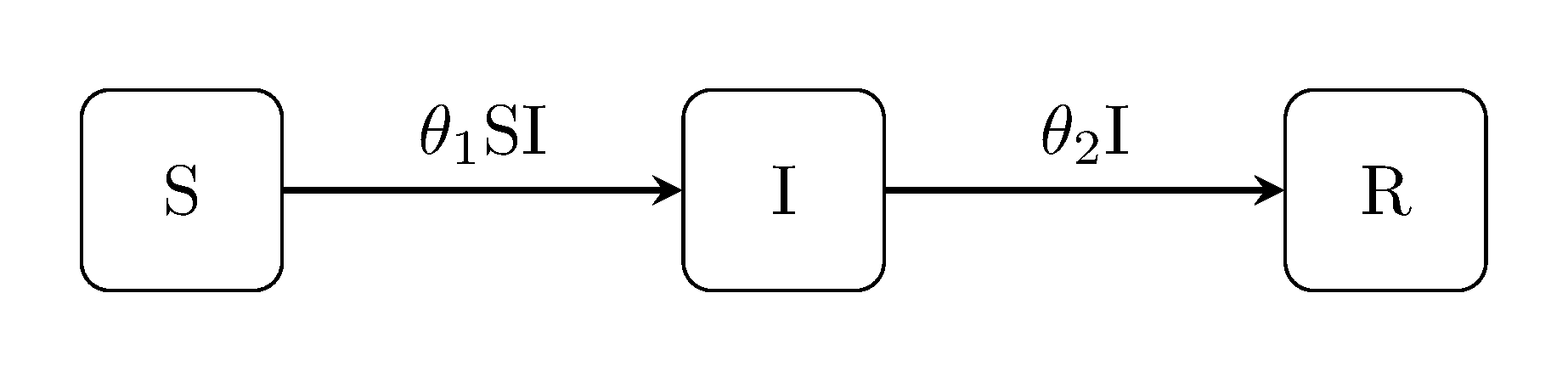
SIR model

The canonical Kermack-McKendrick susceptible-infectious-recovered model is perhaps the best known example of state-space models used within the field of epidemiology.

julia> using DiscretePOMP

julia> generate_model("SIR", [100, 1, 0])
DPOMPModel("SIR", DiscretePOMP.var"#sir_rf#23"(), [100, 1, 0], [-1 1 0; 0 -1 1], DiscretePOMP.dmy_obs_fn, DiscretePOMP.var"#gom2#20"{UnitRange{Int64},UnitRange{Int64},Float64,Float64}(2:2, 2:2, -1.612085713764618, 8.0), Distributions.Product{Distributions.Continuous,Distributions.Uniform{Float64},Array{Distributions.Uniform{Float64},1}}(v=Distributions.Uniform{Float64}[Distributions.Uniform{Float64}(a=0.0, b=1.0), Distributions.Uniform{Float64}(a=0.0, b=1.0)]), 0)

SI model

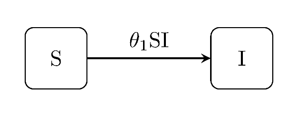
The susceptible-infectious model is the simplest conceptual example of this class of model; two states and only one type of event.

julia> generate_model("SI", [100, 1]);

SIS model

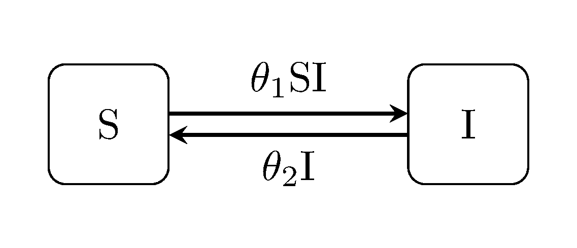
Another common derivative of the SIR model.

julia> generate_model("SIS", [100, 1]);

SEI model

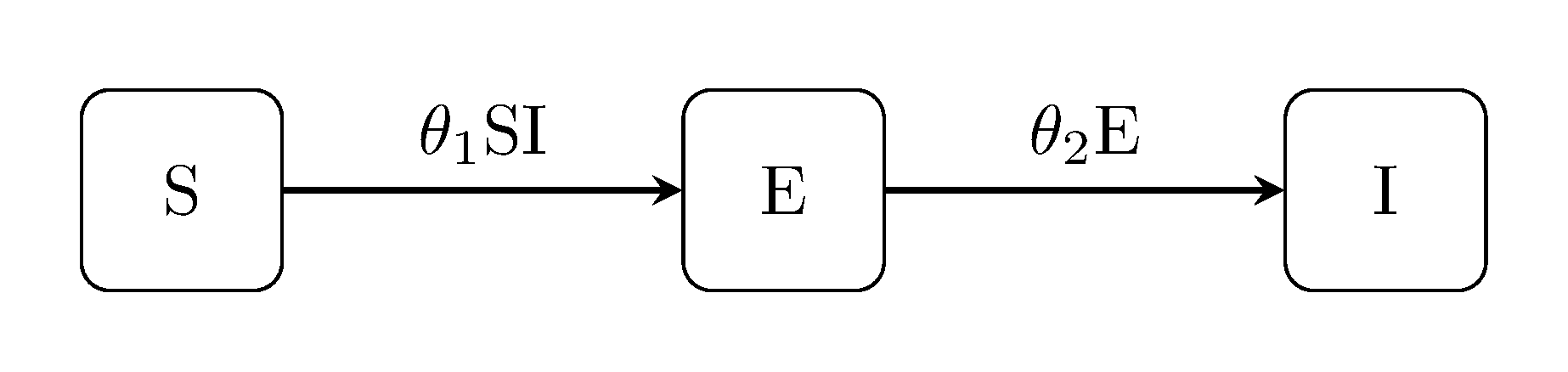
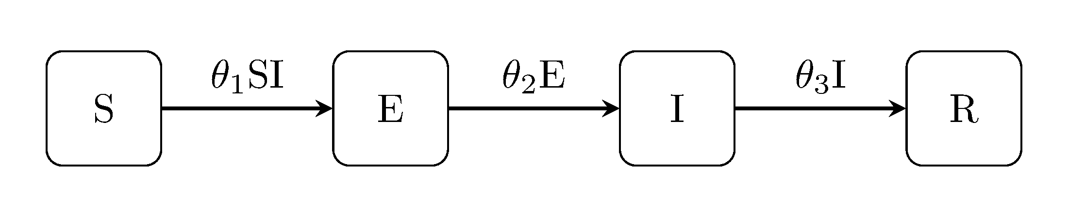
The SEI model includes an 'exposed' state, i.e. for modelling communicable diseases with latent non-infectious periods.

julia> generate_model("SEI", [100, 0, 1]);

SEIR model

Somewhat obviously, the SEIR model concept combines the SEI with the SIR.

julia> generate_model("SEIR", [100, 0, 1, 0]);

Others

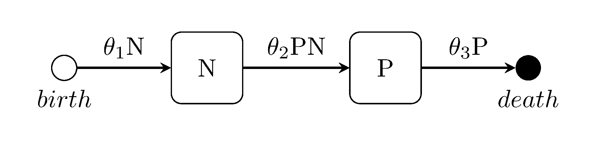
The Lotka-Volterra predator-prey model

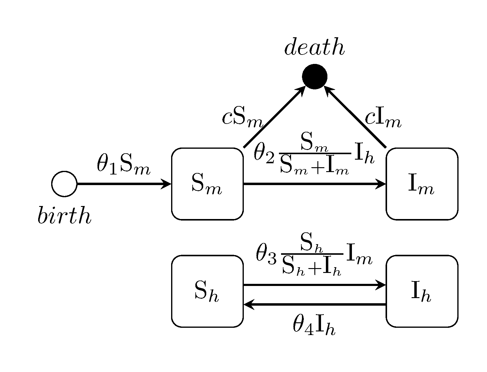
julia> generate_model("LOTKA", [70, 70]);

Ross-MacDonald two-species Malaria model

julia> generate_model("ROSSMAC", [100, 0, 400, 50]);