Constructing Tensors
You can build a finch tensor with the Tensor constructor. In general, the Tensor constructor mirrors Julia's Array constructor, but with an additional prefixed argument which specifies the formatted storage for the tensor.
For example, to construct an empty sparse matrix:
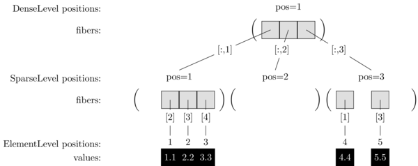
julia> A_fbr = Tensor(Dense(SparseList(Element(0.0))), 4, 3)
4×3-Tensor
└─ Dense [:,1:3]
   ├─ [:, 1]: SparseList (0.0) [1:4]
   ├─ [:, 2]: SparseList (0.0) [1:4]
   └─ [:, 3]: SparseList (0.0) [1:4]
To initialize a sparse matrix with some values:
julia> A = [0.0 0.0 4.4; 1.1 0.0 0.0; 2.2 0.0 5.5; 3.3 0.0 0.0]
4×3 Matrix{Float64}:
 0.0  0.0  4.4
 1.1  0.0  0.0
 2.2  0.0  5.5
 3.3  0.0  0.0

julia> A_fbr = Tensor(Dense(SparseList(Element(0.0))), A)
4×3-Tensor
└─ Dense [:,1:3]
   ├─ [:, 1]: SparseList (0.0) [1:4]
   │  ├─ [2]: 1.1
   │  ├─ [3]: 2.2
   │  └─ [4]: 3.3
   ├─ [:, 2]: SparseList (0.0) [1:4]
   └─ [:, 3]: SparseList (0.0) [1:4]
      ├─ [1]: 4.4
      └─ [3]: 5.5
Storage Tree Level Formats
This section describes the formatted storage for Finch tensors, the first argument to the Tensor constructor. Level storage types holds all of the tensor data, and can be nested hierarchichally.
Finch represents tensors hierarchically in a tree, where each node in the tree is a vector of subtensors and the leaves are the elements. Thus, a matrix is analogous to a vector of vectors, and a 3-tensor is analogous to a vector of vectors of vectors. The vectors at each level of the tensor all have the same structure, which can be selected by the user.
In a Finch tensor tree, the child of each node is selected by an array index. All of the children at the same level will use the same format and share the same storage. Finch is column major, so in an expression A[i_1, ..., i_N], the rightmost dimension i_N corresponds to the root level of the tree, and the leftmost dimension i_1 corresponds to the leaf level.
Our example could be visualized as follows:
Types of Level Storage
Finch supports a variety of storage formats for each level of the tensor tree, each with advantages and disadvantages. Some storage formats support in-order access, while others support random access. Some storage formats must be written to in column-major order, while others support out-of-order writes. The capabilities of each level are summarized in the following tables along with some general descriptions.
| Level Format Name | Group | Data Characteristic | Column-Major Reads | Random Reads | Column-Major Bulk Update | Random Bulk Update | Random Updates | Status |
|---|---|---|---|---|---|---|---|---|
| Dense | Core | Dense | ✅ | ✅ | ✅ | ✅ | ✅ | ✅ |
| SparseTree | Core | Sparse | ✅ | ✅ | ✅ | ✅ | ✅ | ⚙️ |
| SparseRLETree | Core | Sparse Runs | ✅ | ✅ | ✅ | ✅ | ✅ | ⚙️ |
| Element | Core | Leaf | ✅ | ✅ | ✅ | ✅ | ✅ | ✅ |
| Pattern | Core | Leaf | ✅ | ✅ | ✅ | ✅ | ✅ | ✅ |
| SparseList | Advanced | Sparse | ✅ | ❌ | ✅ | ❌ | ❌ | ✅ |
| SparseRLE | Advanced | Sparse Runs | ✅ | ❌ | ✅ | ❌ | ❌ | ✅ |
| SparseVBL | Advanced | Sparse Blocks | ✅ | ❌ | ✅ | ❌ | ❌ | ✅ |
| SparsePoint | Advanced | Single Sparse | ✅ | ✅ | ✅ | ❌ | ❌ | ✅ |
| SparseInterval | Advanced | Single Sparse Run | ✅ | ✅ | ✅ | ❌ | ❌ | ✅ |
| SparseBand | Advanced | Single Sparse Block | ✅ | ✅ | ✅ | ❌ | ❌ | ⚙️ |
| DenseRLE | Advanced | Dense Runs | ✅ | ❌ | ✅ | ❌ | ❌ | ⚙ |
| SparseBytemap | Advanced | Sparse | ✅ | ✅ | ✅ | ✅ | ❌ | ✅ |
| SparseDict | Advanced | Sparse | ✅ | ✅ | ✅ | ✅ | ❌ | ✅️ |
| AtomicLevel | Modifier | No Data | ✅ | ✅ | ✅ | ✅ | ✅ | ⚙️ |
| SeperationLevel | Modifier | No Data | ✅ | ✅ | ✅ | ✅ | ✅ | ⚙️ |
| SparseCOO | Legacy | Sparse | ✅ | ✅ | ✅ | ❌ | ✅ | ✅️ |
The "Level Format Name" is the name of the level datatype. Other columns have descriptions below.
Status
| Symbol | Meaning |
|---|---|
| ✅ | Indicates the level is ready for serious use. |
| ⚙️ | Indicates the level is experimental and under development. |
| 🕸️ | Indicates the level is deprecated, and may be removed in a future release. |
Groups
Core Group
Contains the basic, minimal set of levels one should use to build and manipulate tensors. These levels can be efficiently read and written to in any order.
Advanced Group
Contains levels which are more specialized, and geared towards bulk updates. These levels may be more efficient in certain cases, but are also more restrictive about access orders and intended for more advanced usage.
Modifier Group
Contains levels which are also more specialized, but not towards a sparsity pattern. These levels modify other levels in a variety of ways, but don't store novel sparsity patterns. Typically, they modify how levels are stored or attach data to levels to support the utilization of various hardware features.
Legacy Group
Contains levels which are not recommended for new code, but are included for compatibility with older code.
Data Characteristics
| Level Type | Description |
|---|---|
| Dense | Levels which store every subtensor. |
| Leaf | Levels which store only scalars, used for the leaf level of the tree. |
| Sparse | Levels which store only non-fill values, used for levels with few nonzeros. |
| Sparse Runs | Levels which store runs of repeated non-fill values. |
| Sparse Blocks | Levels which store Blocks of repeated non-fill values. |
| Dense Runs | Levels which store runs of repeated values, and no compile-time zero annihilation. |
| No Data | Levels which don't store data but which alter the storage pattern or attach additional meta-data. |
Note that the Single sparse levels store a single instance of each nonzero, run, or block. These are useful with a parent level to represent IDs.
Access Characteristics
| Operation Type | Description |
|---|---|
| Column-Major Reads | Indicates efficient reading of data in column-major order. |
| Random Reads | Indicates efficient reading of data in random-access order. |
| Column-Major Bulk Update | Indicates efficient writing of data in column-major order, the total time roughly linear to the size of the tensor. |
| Column-Major Random Update | Indicates efficient writing of data in random-access order, the total time roughly linear to the size of the tensor. |
| Random Update | Indicates efficient writing of data in random-access order, the total time roughly linear to the number of updates. |
Examples of Popular Formats in Finch
Finch levels can be used to construct a variety of popular sparse formats. A few examples follow:
| Format Type | Syntax |
|---|---|
| Sparse Vector | Tensor(SparseList(Element(0.0)), args...) |
| CSC Matrix | Tensor(Dense(SparseList(Element(0.0))), args...) |
| CSF 3-Tensor | Tensor(Dense(SparseList(SparseList(Element(0.0)))), args...) |
| DCSC (Hypersparse) Matrix | Tensor(SparseList(SparseList(Element(0.0))), args...) |
| COO Matrix | Tensor(SparseCOO{2}(Element(0.0)), args...) |
| COO 3-Tensor | Tensor(SparseCOO{3}(Element(0.0)), args...) |
| Run-Length-Encoded Image | Tensor(Dense(DenseRLE(Element(0.0))), args...) |
Tensor Constructors
Finch.Tensor — TypeTensor{Lvl} <: AbstractFiber{Lvl}The multidimensional array type used by Finch. Tensor is a thin wrapper around the hierarchical level storage of type Lvl.
Finch.Tensor — MethodTensor(lvl)Construct a Tensor using the tensor level storage lvl. No initialization of storage is performed, it is assumed that position 1 of lvl corresponds to a valid tensor, and lvl will be wrapped as-is. Call a different constructor to initialize the storage.
Finch.Tensor — MethodTensor(lvl, [undef], dims...)Construct a Tensor of size dims, and initialize to undef, potentially allocating memory. Here undef is the UndefInitializer singleton type. dims... may be a variable number of dimensions or a tuple of dimensions, but it must correspond to the number of dimensions in lvl.
Finch.Tensor — MethodTensor(lvl, arr)Construct a Tensor and initialize it to the contents of arr. To explicitly copy into a tensor, use @ref[copyto!]
Finch.Tensor — MethodTensor(lvl, arr)Construct a Tensor and initialize it to the contents of arr. To explicitly copy into a tensor, use @ref[copyto!]
Finch.Tensor — MethodTensor(arr, [init = zero(eltype(arr))])Copy an array-like object arr into a corresponding, similar Tensor datastructure. Uses init as an initial value. May reuse memory when possible. To explicitly copy into a tensor, use @ref[copyto!].
Examples
julia> println(summary(Tensor(sparse([1 0; 0 1]))))
2×2 Tensor(Dense(SparseList(Element(0))))

julia> println(summary(Tensor(ones(3, 2, 4))))
3×2×4 Tensor(Dense(Dense(Dense(Element(0.0)))))
Level Constructors
Core Levels
Finch.DenseLevel — TypeDenseLevel{[Ti=Int]}(lvl, [dim])A subfiber of a dense level is an array which stores every slice A[:, ..., :, i] as a distinct subfiber in lvl. Optionally, dim is the size of the last dimension. Ti is the type of the indices used to index the level.
julia> ndims(Tensor(Dense(Element(0.0))))
1

julia> ndims(Tensor(Dense(Dense(Element(0.0)))))
2

julia> Tensor(Dense(Dense(Element(0.0))), [1 2; 3 4])
2×2-Tensor
└─ Dense [:,1:2]
   ├─ [:, 1]: Dense [1:2]
   │  ├─ [1]: 1.0
   │  └─ [2]: 3.0
   └─ [:, 2]: Dense [1:2]
      ├─ [1]: 2.0
      └─ [2]: 4.0
Finch.ElementLevel — TypeElementLevel{Vf, [Tv=typeof(Vf)], [Tp=Int], [Val]}()A subfiber of an element level is a scalar of type Tv, initialized to Vf. Vf may optionally be given as the first argument.
The data is stored in a vector of type Val with eltype(Val) = Tv. The type Tp is the index type used to access Val.
julia> Tensor(Dense(Element(0.0)), [1, 2, 3])
3-Tensor
└─ Dense [1:3]
   ├─ [1]: 1.0
   ├─ [2]: 2.0
   └─ [3]: 3.0
Finch.PatternLevel — TypePatternLevel{[Tp=Int]}()A subfiber of a pattern level is the Boolean value true, but it's fill_value is false. PatternLevels are used to create tensors that represent which values are stored by other fibers. See pattern! for usage examples.
julia> Tensor(Dense(Pattern()), 3)
3-Tensor
└─ Dense [1:3]
   ├─ [1]: true
   ├─ [2]: true
   └─ [3]: true
Advanced Levels
Finch.SparseListLevel — TypeSparseListLevel{[Ti=Int], [Ptr, Idx]}(lvl, [dim])A subfiber of a sparse level does not need to represent slices A[:, ..., :, i] which are entirely fill_value. Instead, only potentially non-fill slices are stored as subfibers in lvl. A sorted list is used to record which slices are stored. Optionally, dim is the size of the last dimension.
Ti is the type of the last tensor index, and Tp is the type used for positions in the level. The types Ptr and Idx are the types of the arrays used to store positions and indicies.
julia> Tensor(Dense(SparseList(Element(0.0))), [10 0 20; 30 0 0; 0 0 40])
3×3-Tensor
└─ Dense [:,1:3]
   ├─ [:, 1]: SparseList (0.0) [1:3]
   │  ├─ [1]: 10.0
   │  └─ [2]: 30.0
   ├─ [:, 2]: SparseList (0.0) [1:3]
   └─ [:, 3]: SparseList (0.0) [1:3]
      ├─ [1]: 20.0
      └─ [3]: 40.0

julia> Tensor(SparseList(SparseList(Element(0.0))), [10 0 20; 30 0 0; 0 0 40])
3×3-Tensor
└─ SparseList (0.0) [:,1:3]
   ├─ [:, 1]: SparseList (0.0) [1:3]
   │  ├─ [1]: 10.0
   │  └─ [2]: 30.0
   └─ [:, 3]: SparseList (0.0) [1:3]
      ├─ [1]: 20.0
      └─ [3]: 40.0
Finch.DenseRLELevel — TypeDenseRLELevel{[Ti=Int], [Ptr, Right]}(lvl, [dim], [merge = true])The dense RLE level represent runs of equivalent slices A[:, ..., :, i]. A sorted list is used to record the right endpoint of each run. Optionally, dim is the size of the last dimension.
Ti is the type of the last tensor index, and Tp is the type used for positions in the level. The types Ptr and Right are the types of the arrays used to store positions and endpoints.
The merge keyword argument is used to specify whether the level should merge duplicate consecutive runs.
julia> Tensor(Dense(DenseRLELevel(Element(0.0))), [10 0 20; 30 0 0; 0 0 40])
3×3-Tensor
└─ Dense [:,1:3]
   ├─ [:, 1]: DenseRLE (0.0) [1:3]
   │  ├─ [1:1]: 10.0
   │  ├─ [2:2]: 30.0
   │  └─ [3:3]: 0.0
   ├─ [:, 2]: DenseRLE (0.0) [1:3]
   │  └─ [1:3]: 0.0
   └─ [:, 3]: DenseRLE (0.0) [1:3]
      ├─ [1:1]: 20.0
      ├─ [2:2]: 0.0
      └─ [3:3]: 40.0
Finch.SparseRLELevel — TypeSparseRLELevel{[Ti=Int], [Ptr, Left, Right]}(lvl, [dim]; [merge = true])The sparse RLE level represent runs of equivalent slices A[:, ..., :, i] which are not entirely fill_value. A sorted list is used to record the left and right endpoints of each run. Optionally, dim is the size of the last dimension.
Ti is the type of the last tensor index, and Tp is the type used for positions in the level. The types Ptr, Left, and Right are the types of the arrays used to store positions and endpoints.
The merge keyword argument is used to specify whether the level should merge duplicate consecutive runs.
julia> Tensor(Dense(SparseRLELevel(Element(0.0))), [10 0 20; 30 0 0; 0 0 40])
3×3-Tensor
└─ Dense [:,1:3]
   ├─ [:, 1]: SparseRLE (0.0) [1:3]
   │  ├─ [1:1]: 10.0
   │  └─ [2:2]: 30.0
   ├─ [:, 2]: SparseRLE (0.0) [1:3]
   └─ [:, 3]: SparseRLE (0.0) [1:3]
      ├─ [1:1]: 20.0
      └─ [3:3]: 40.0
Finch.SparseVBLLevel — TypeSparseVBLLevel{[Ti=Int], [Ptr, Idx, Ofs]}(lvl, [dim])
Like the SparseListLevel, but contiguous subfibers are stored together in blocks.
```jldoctest julia> Tensor(Dense(SparseVBL(Element(0.0))), [10 0 20; 30 0 0; 0 0 40]) Dense [:,1:3] ├─[:,1]: SparseList (0.0) [1:3] │ ├─[1]: 10.0 │ ├─[2]: 30.0 ├─[:,2]: SparseList (0.0) [1:3] ├─[:,3]: SparseList (0.0) [1:3] │ ├─[1]: 20.0 │ ├─[3]: 40.0
julia> Tensor(SparseVBL(SparseVBL(Element(0.0))), [10 0 20; 30 0 0; 0 0 40]) SparseList (0.0) [:,1:3] ├─[:,1]: SparseList (0.0) [1:3] │ ├─[1]: 10.0 │ ├─[2]: 30.0 ├─[:,3]: SparseList (0.0) [1:3] │ ├─[1]: 20.0 │ ├─[3]: 40.0
Finch.SparseBandLevel — TypeSparseBandLevel{[Ti=Int], [Ptr, Idx, Ofs]}(lvl, [dim])
Like the SparseVBLLevel, but stores only a single block, and fills in zeros.
```jldoctest julia> Tensor(Dense(SparseBand(Element(0.0))), [10 0 20; 30 40 0; 0 0 50]) Dense [:,1:3] ├─[:,1]: SparseList (0.0) [1:3] │ ├─[1]: 10.0 │ ├─[2]: 30.0 ├─[:,2]: SparseList (0.0) [1:3] ├─[:,3]: SparseList (0.0) [1:3] │ ├─[1]: 20.0 │ ├─[3]: 40.0
Finch.SparsePointLevel — TypeSparsePointLevel{[Ti=Int], [Ptr, Idx]}(lvl, [dim])A subfiber of a SparsePoint level does not need to represent slices A[:, ..., :, i] which are entirely fill_value. Instead, only potentially non-fill slices are stored as subfibers in lvl. A main difference compared to SparseList level is that SparsePoint level only stores a 'single' non-fill slice. It emits an error if the program tries to write multiple (>=2) coordinates into SparsePoint.
Ti is the type of the last tensor index. The types Ptr and Idx are the types of the arrays used to store positions and indicies.
julia> Tensor(Dense(SparsePoint(Element(0.0))), [10 0 0; 0 20 0; 0 0 30])
3×3-Tensor
└─ Dense [:,1:3]
   ├─ [:, 1]: SparsePoint (0.0) [1:3]
   │  └─ 10.0
   ├─ [:, 2]: SparsePoint (0.0) [1:3]
   │  └─ 20.0
   └─ [:, 3]: SparsePoint (0.0) [1:3]
      └─ 30.0

julia> Tensor(SparsePoint(Dense(Element(0.0))), [0 0 0; 0 0 30; 0 0 30])
3×3-Tensor
└─ SparsePoint (0.0) [:,1:3]
   └─ Dense [1:3]
      ├─ [1]: 0.0
      ├─ [2]: 30.0
      └─ [3]: 30.0
Finch.SparseIntervalLevel — TypeSparseIntervalLevel{[Ti=Int], [Ptr, Left, Right]}(lvl, [dim])The single RLE level represent runs of equivalent slices A[:, ..., :, i] which are not entirely fill_value. A main difference compared to SparseRLE level is that SparseInterval level only stores a 'single' non-fill run. It emits an error if the program tries to write multiple (>=2) runs into SparseInterval.
Ti is the type of the last tensor index. The types Ptr, Left, and 'Right' are the types of the arrays used to store positions and endpoints.
julia> Tensor(SparseInterval(Element(0)), [0, 10, 0])
3-Tensor
└─ SparseInterval (0) [1:3]
   └─ [2:2]: 10

julia> x = Tensor(SparseInterval(Element(0)), 10);

julia> @finch begin for i = extent(3,6); x[~i] = 1 end end;

julia> x
10-Tensor
└─ SparseInterval (0) [1:10]
   └─ [3:6]: 1
Finch.SparseByteMapLevel — TypeSparseByteMapLevel{[Ti=Int], [Ptr, Tbl]}(lvl, [dims])Like the SparseListLevel, but a dense bitmap is used to encode which slices are stored. This allows the ByteMap level to support random access.
Ti is the type of the last tensor index, and Tp is the type used for positions in the level.
julia> Tensor(Dense(SparseByteMap(Element(0.0))), [10 0 20; 30 0 0; 0 0 40])
3×3-Tensor
└─ Dense [:,1:3]
   ├─ [:, 1]: SparseByteMap (0.0) [1:3]
   │  ├─ [1]: 10.0
   │  └─ [2]: 30.0
   ├─ [:, 2]: SparseByteMap (0.0) [1:3]
   └─ [:, 3]: SparseByteMap (0.0) [1:3]
      ├─ [1]: 0.0
      └─ [3]: 0.0

julia> Tensor(SparseByteMap(SparseByteMap(Element(0.0))), [10 0 20; 30 0 0; 0 0 40])
3×3-Tensor
└─ SparseByteMap (0.0) [:,1:3]
   ├─ [:, 1]: SparseByteMap (0.0) [1:3]
   │  ├─ [1]: 10.0
   │  └─ [2]: 30.0
   └─ [:, 3]: SparseByteMap (0.0) [1:3]
Finch.SparseDictLevel — TypeSparseDictLevel{[Ti=Int], [Tp=Int], [Ptr, Idx, Val, Tbl, Pool=Dict]}(lvl, [dim])A subfiber of a sparse level does not need to represent slices A[:, ..., :, i] which are entirely fill_value. Instead, only potentially non-fill slices are stored as subfibers in lvl. A datastructure specified by Tbl is used to record which slices are stored. Optionally, dim is the size of the last dimension.
Ti is the type of the last fiber index, and Tp is the type used for positions in the level. The types Ptr and Idx are the types of the arrays used to store positions and indicies.
julia> Tensor(Dense(SparseDict(Element(0.0))), [10 0 20; 30 0 0; 0 0 40])
3×3-Tensor
└─ Dense [:,1:3]
   ├─ [:, 1]: SparseDict (0.0) [1:3]
   │  ├─ [1]: 10.0
   │  └─ [2]: 30.0
   ├─ [:, 2]: SparseDict (0.0) [1:3]
   └─ [:, 3]: SparseDict (0.0) [1:3]
      ├─ [1]: 20.0
      └─ [3]: 40.0

julia> Tensor(SparseDict(SparseDict(Element(0.0))), [10 0 20; 30 0 0; 0 0 40])
3×3-Tensor
└─ SparseDict (0.0) [:,1:3]
   ├─ [:, 1]: SparseDict (0.0) [1:3]
   │  ├─ [1]: 10.0
   │  └─ [2]: 30.0
   └─ [:, 3]: SparseDict (0.0) [1:3]
      ├─ [1]: 20.0
      └─ [3]: 40.0
Modifier Levels
Finch.SeparateLevel — TypeSeparateLevel{Lvl, [Val]}()A subfiber of a Separate level is a separate tensor of type Lvl, in it's own memory space.
Each sublevel is stored in a vector of type Val with eltype(Val) = Lvl.
julia> Tensor(Dense(Separate(Element(0.0))), [1, 2, 3])
3-Tensor
└─ Dense [1:3]
   ├─ [1]: Pointer ->
   │  └─ 1.0
   ├─ [2]: Pointer ->
   │  └─ 2.0
   └─ [3]: Pointer ->
      └─ 3.0
Legacy Levels
Finch.SparseCOOLevel — TypeSparseCOOLevel{[N], [TI=Tuple{Int...}], [Ptr, Tbl]}(lvl, [dims])A subfiber of a sparse level does not need to represent slices which are entirely fill_value. Instead, only potentially non-fill slices are stored as subfibers in lvl. The sparse coo level corresponds to N indices in the subfiber, so fibers in the sublevel are the slices A[:, ..., :, i_1, ..., i_n]. A set of N lists (one for each index) are used to record which slices are stored. The coordinates (sets of N indices) are sorted in column major order. Optionally, dims are the sizes of the last dimensions.
TI is the type of the last N tensor indices, and Tp is the type used for positions in the level.
The type Tbl is an NTuple type where each entry k is a subtype AbstractVector{TI[k]}.
The type Ptr is the type for the pointer array.
julia> Tensor(Dense(SparseCOO{1}(Element(0.0))), [10 0 20; 30 0 0; 0 0 40])
3×3-Tensor
└─ Dense [:,1:3]
   ├─ [:, 1]: SparseCOO{1} (0.0) [1:3]
   │  ├─ [1]: 10.0
   │  └─ [2]: 30.0
   ├─ [:, 2]: SparseCOO{1} (0.0) [1:3]
   └─ [:, 3]: SparseCOO{1} (0.0) [1:3]
      ├─ [1]: 20.0
      └─ [3]: 40.0

julia> Tensor(SparseCOO{2}(Element(0.0)), [10 0 20; 30 0 0; 0 0 40])
3×3-Tensor
└─ SparseCOO{2} (0.0) [:,1:3]
   ├─ [1, 1]: 10.0
   ├─ [2, 1]: 30.0
   ├─ [1, 3]: 20.0
   └─ [3, 3]: 40.0