Examples

Birth-Death Model

This example models a linear birth-death process. The reaction network is easily defined using Catalyst.jl. Our truncated state space has length 50, which is enough for this simple system.

using FiniteStateProjection
using OrdinaryDiffEq

rn = @reaction_network begin
    σ, 0 --> A
    d, A --> 0
end

sys = FSPSystem(rn)

# Parameters for our system
ps = [ 10.0, 1.0 ]

# Initial distribution (over 1 species)
# Here we start with 0 copies of A
u0 = zeros(50)
u0[1] = 1.0

prob = ODEProblem(sys, u0, (0, 10.0), ps)
sol = solve(prob, Vern7())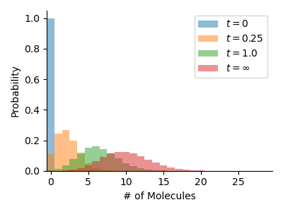

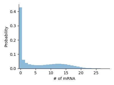
Telegraph Model

Here we showcase the telegraph model, a simplistic description of mRNA transcription in biological cells. We have one gene that transitions stochastically between an on and an off state and produces mRNA molecules while it is in the on state.

The most straightforward description of this system includes three species: two gene states, G_on and G_off, and mRNA M. The state space for this system is 3-dimensional. We know, however, that G_on and G_off never occur at the same time, indeed the conservation law [G_on] + [G_off] = 1 allows us to express the state of the system in terms of G_on and M only. The state space of this reduced system is 2-dimensional.If we use an mRNA cutoff of 100, the state space for the original model has size $2 \times 2 \times 100 = 400$, while the reduced state space has size $2 \times 100 = 200$, a two-fold saving. Since the FSP get computationally more expensive for each species in a system, eliminating redundant species as above is recommended for improved performance.

using FiniteStateProjection
using OrdinaryDiffEq

rn = @reaction_network begin
    σ_on * (1 - G_on), 0 --> G_on
    σ_off, G_on --> 0
    ρ, G_on --> G_on + M
    d, M --> 0
end

sys = FSPSystem(rn)

# Parameters for our system
ps = [ 0.25, 0.15, 15.0, 1.0 ]

# Initial distribution (over two species)
# Here we start with 0 copies of G_on and M
u0 = zeros(2, 50)
u0[1,1] = 1.0

prob = ODEProblem(sys, u0, (0, 10.0), ps)
sol = solve(prob, Vern7())