Profiling

Profiling GPU code is harder than profiling Julia code executing on the CPU. For one, kernels typically execute asynchronously, and thus require appropriate synchronization when measuring their execution time. Furthermore, because the code executes on a different processor, it is much harder to know what is currently executing. CUDA, and the Julia CUDA packages, provide several tools and APIs to remedy this.

Time measurements

To accurately measure execution time in the presence of asynchronously-executing kernels, CUDA.jl provides an @elapsed macro that, much like Base.@elapsed, measures the total execution time of a block of code on the GPU:

julia> a = CUDA.rand(1024,1024,1024);

julia> Base.@elapsed sin.(a)  # WRONG!
0.008714211

julia> CUDA.@elapsed sin.(a)
0.051607586f0

This macro is a low-level utility, assumes the GPU is synchronized before calling, and is useful if you need execution timings in your application. For most purposes, you should use CUDA.@time which mimics Base.@time by printing execution times as well as memory allocation stats:

julia> a = CUDA.rand(1024,1024,1024);

julia> CUDA.@time sin.(a);
  0.046063 seconds (96 CPU allocations: 3.750 KiB) (1 GPU allocation: 4.000 GiB, 14.33% gc time of which 99.89% spent allocating)

The @time macro is more user-friendly (synchronizes the GPU before measuring so you don't need to do a thing), uses wall-clock time, and is a generally more useful tool when measuring the end-to-end performance characteristics of a GPU application.

For robust measurements however, it is advised to use the BenchmarkTools.jl package which goes to great lengths to perform accurate measurements. Due to the asynchronous nature of GPUs, you need to ensure the GPU is synchronized at the end of every sample, e.g. by calling synchronize(). An easier, and better-performing alternative is to use the unexported @sync macro:

julia> a = CUDA.rand(1024,1024,1024);

julia> @benchmark CUDA.@sync sin.($a)
BenchmarkTools.Trial:
  memory estimate:  3.73 KiB
  allocs estimate:  95
  --------------
  minimum time:     46.341 ms (0.00% GC)
  median time:      133.302 ms (0.50% GC)
  mean time:        130.087 ms (0.49% GC)
  maximum time:     153.465 ms (0.43% GC)
  --------------
  samples:          39
  evals/sample:     1

Note that the allocations as reported by BenchmarkTools are CPU allocations. For the GPU allocation behavior you need to consult CUDA.@time.

Application profiling

For profiling large applications, simple timings are insufficient. Instead, we want a overview of how and when the GPU was active, to avoid times where the device was idle and/or find which kernels needs optimization.

As we cannot use the Julia profiler for this task, we will be using external profiling software as part of the CUDA toolkit. To inform those external tools which code needs to be profiled (e.g., to exclude warm-up iterations or other noninteresting elements) you can use the CUDA.@profile macro to surround interesting code with. Again, this macro mimics an equivalent from the standard library, but this time requires external software to actually perform the profiling:

julia> a = CUDA.rand(1024,1024,1024);

julia> sin.(a);  # warmup

julia> CUDA.@profile sin.(a);
┌ Warning: Calling CUDA.@profile only informs an external profiler to start.
│ The user is responsible for launching Julia under a CUDA profiler like `nvprof`.
└ @ CUDA.Profile ~/Julia/pkg/CUDA/src/profile.jl:42

nvprof and nvvp

For simple profiling, prefix your Julia command-line invocation with the nvprof utility. For a better timeline, be sure to use CUDA.@profile to delimit interesting code and start nvprof with the option --profile-from-start off:

$ nvprof --profile-from-start off julia

julia> using CUDA

julia> a = CUDA.rand(1024,1024,1024);

julia> sin.(a);

julia> CUDA.@profile sin.(a);

julia> exit()
==156406== Profiling application: julia
==156406== Profiling result:
            Type  Time(%)      Time     Calls       Avg       Min       Max  Name
 GPU activities:  100.00%  44.777ms         1  44.777ms  44.777ms  44.777ms  ptxcall_broadcast_1
      API calls:   56.46%  6.6544ms         1  6.6544ms  6.6544ms  6.6544ms  cuMemAlloc
                   43.52%  5.1286ms         1  5.1286ms  5.1286ms  5.1286ms  cuLaunchKernel
                    0.01%  1.3200us         1  1.3200us  1.3200us  1.3200us  cuDeviceGetCount
                    0.01%     725ns         3     241ns     196ns     301ns  cuCtxGetCurrent

For a visual overview of these results, you can use the NVIDIA Visual Profiler (nvvp):

Note however that both nvprof and nvvp are deprecated, and will be removed from future versions of the CUDA toolkit.

NVIDIA Nsight Systems

Following the deprecation of above tools, NVIDIA published the Nsight Systems and Nsight Compute tools for respectively timeline profiling and more detailed kernel analysis. The former is well-integrated with the Julia GPU packages, and makes it possible to iteratively profile without having to restart Julia as was the case with nvvp and nvprof.

After downloading and installing NSight Systems (a version might have been installed alongside with the CUDA toolkit, but it is recommended to download and install the latest version from the NVIDIA website), you need to launch Julia from the command-line, wrapped by the nsys utility from NSight Systems:

$ nsys launch julia

You can then execute whatever code you want in the REPL, including e.g. loading Revise so that you can modify your application as you go. When you call into code that is wrapped by CUDA.@profile, the profiler will become active and generate a profile output file in the current folder:

julia> using CUDA

julia> a = CUDA.rand(1024,1024,1024);

julia> sin.(a);

julia> CUDA.@profile sin.(a);
start executed
Processing events...
Capturing symbol files...
Saving intermediate "report.qdstrm" file to disk...

Importing [===============================================================100%]
Saved report file to "report.qdrep"
stop executed

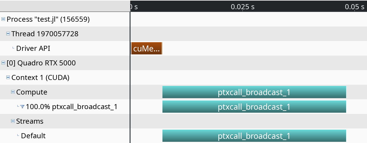
You can open the resulting .qdrep file with nsight-sys:

NVIDIA Nsight Compute

If you want details on the execution properties of a kernel, or inspect API interactions, Nsight Compute is the tool for you. It is again possible to use this profiler with an interactive session of Julia, and debug or profile only those sections of your application that are marked with CUDA.@profile.

Start with launching Julia under the Nsight Compute CLI tool:

$ nv-nsight-cu-cli --mode=launch julia

You will get an interactive REPL, where you can execute whatever code you want:

julia> using CUDA

# Julia hangs!

As soon as you import CUDA.jl, your Julia process will hang. This is expected, as the tool breaks upon the very first call to the CUDA API, at which point you are expected to launch the Nsight Compute GUI utility and attach to the running session:

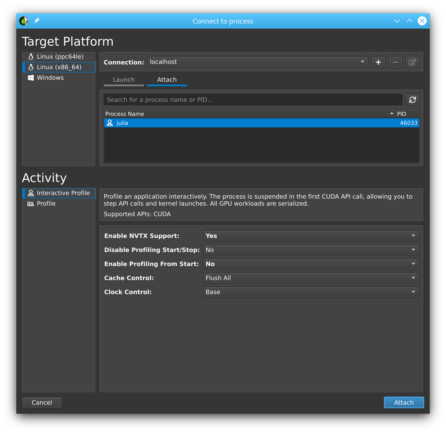
You will see that the tool has stopped execution on the call to cuInit. Now check Profile > Auto Profile to make Nsight Compute gather statistics on our kernels, and clock Debug > Resume to resume your session.

Now our CLI session comes to life again, and we can enter the rest of our script:

julia> a = CUDA.rand(1024,1024,1024);

julia> sin.(a);

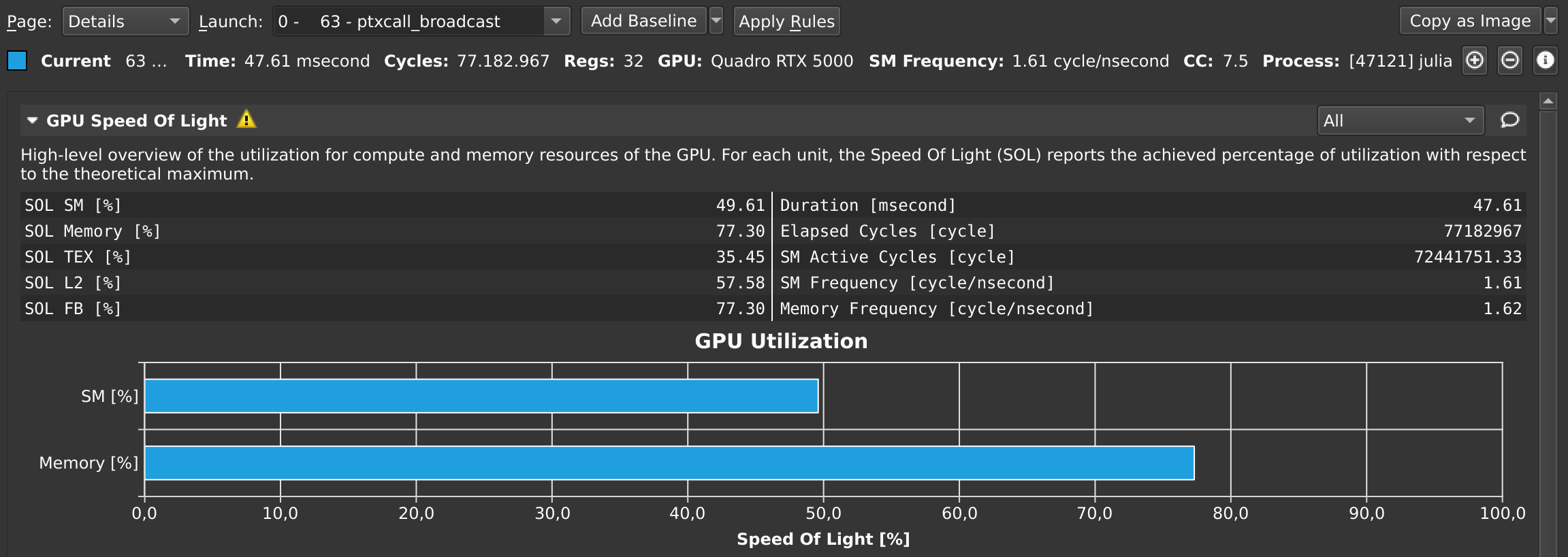
julia> CUDA.@profile sin.(a);

Once that's finished, the Nsight Compute GUI window will have plenty details on our kernel:

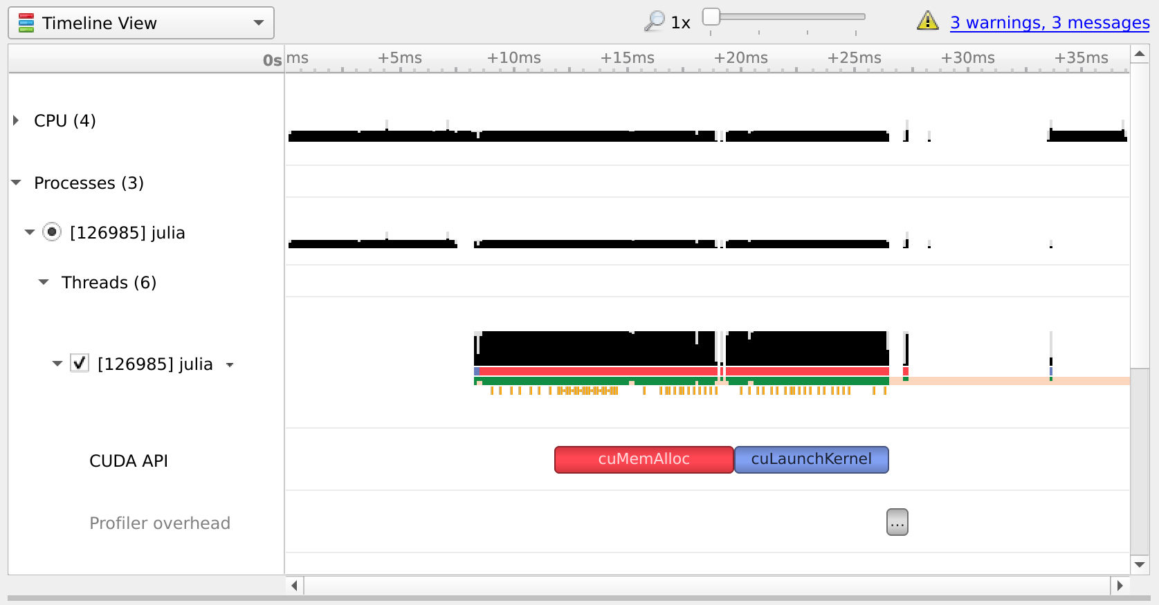
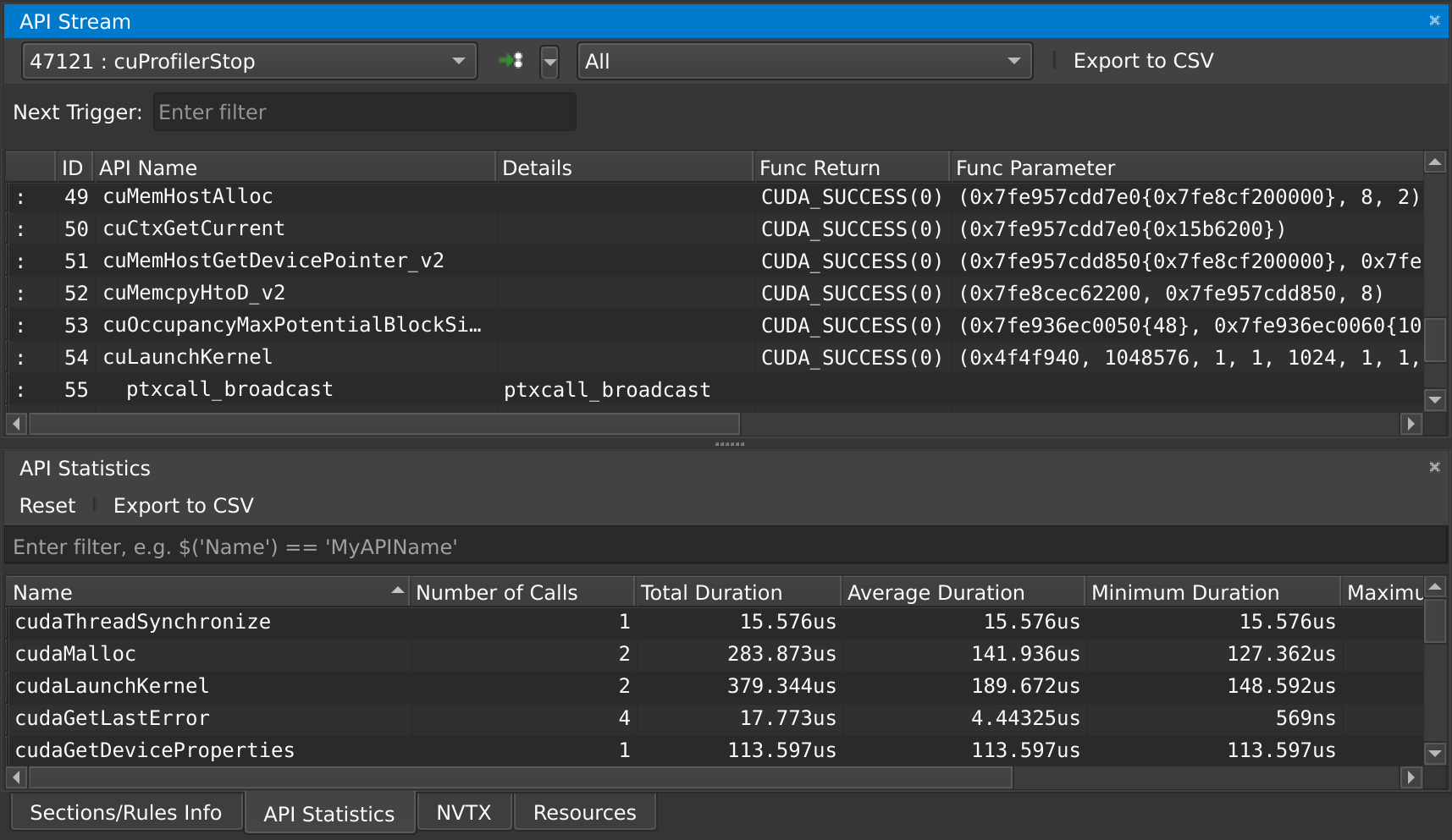
At any point in time, you can also pause your application from the debug menu, and inspect the API calls that have been made:

Source-code annotations

If you want to put additional information in the profile, e.g. phases of your application, or expensive CPU operations, you can use the NVTX library. Wrappers for this library are included in recent versions of CUDA.jl:

using CUDA

NVTX.@range "doing X" begin
    ...
end

NVTX.@mark "reached Y"

Compiler options

Some tools, like nvvp and NSight Systems Compute, also make it possible to do source-level profiling. CUDA.jl will by default emit the necessary source line information, which you can disable by launching Julia with -g0. Conversely, launching with -g2 will emit additional debug information, which can be useful in combination with tools like cuda-gdb, but might hurt performance or code size.