Contours
This guide shows a few different ways to measure and visualize contours of images.
Using Plots
The most basic way to create a contour plot is simply to use Plots.jl contour and contourf functions on your image.
Let's see how that works:
using AstroImages, Plots


# First load a FITS file of interest
fname = download(
    "http://www.astro.uvic.ca/~wthompson/astroimages/fits/herca/herca_radio.fits",
    "herca-radio.fits"
)

herca = load("herca-radio.fits")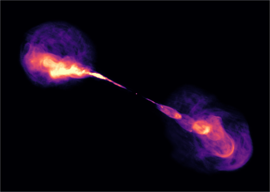
Create a contour plot
contour(herca)
Create a filled contour plot
contourf(herca)
Specify the number of levels
contour(herca, levels=5)
Specify specific levels
contour(herca, levels=[1, 1000, 5000])
Overplot contours on image:
implot(herca)
contour!(herca, levels=4, color=:cyan)
Using Contour.jl
For more control over how contours are calculated and plotted, you can use the Contour.jl package:
using Contour
herca = load("herca-radio.fits")

p = implot(herca, cmap=nothing, colorbar=false)

# Note: Contour.jl only supports float inputs.
# See https://github.com/JuliaGeometry/Contour.jl/issues/73
for cl in levels(contours(dims(herca)..., float.(herca)))
    lvl = level(cl) # the z-value of this contour level
    for line in lines(cl)
        xs, ys = coordinates(line) # coordinates of this line segment
        plot!(p, xs, ys, line_z=lvl, label="")
    end
end

p
Here we plot just the contours, now in world coordinates:
p = plot(xlabel="RA", ylabel="DEC")
for cl in levels(contours(dims(herca)..., float.(herca)))
    lvl = level(cl) # the z-value of this contour level
    for line in lines(cl)
        xs, ys = coordinates(line) # coordinates of this line segment
        worldcoords = map(zip(xs,ys)) do pixcoord
            pix_to_world(herca, [pixcoord...])
        end
        plot!(p, getindex.(worldcoords,1), getindex.(worldcoords,2), line_z=lvl, label="")
    end
end
p