Converting From RGB Images
If you encouter an image in a standard graphics format (e.g. PNG, JPG) that you want to analyze or store in an AstroImage, it will likely contain RGB (or similar) pixels.
It is possible to store RGB data in an AstroImage. Let's see how that works:
using AstroImages
download("http://www.astro.uvic.ca/~wthompson/astroimages/fits/mw-crop2-small.png","mw-crop2-small.png")

# First we load it from the PNG file
mw_png = load("mw-crop2-small.png")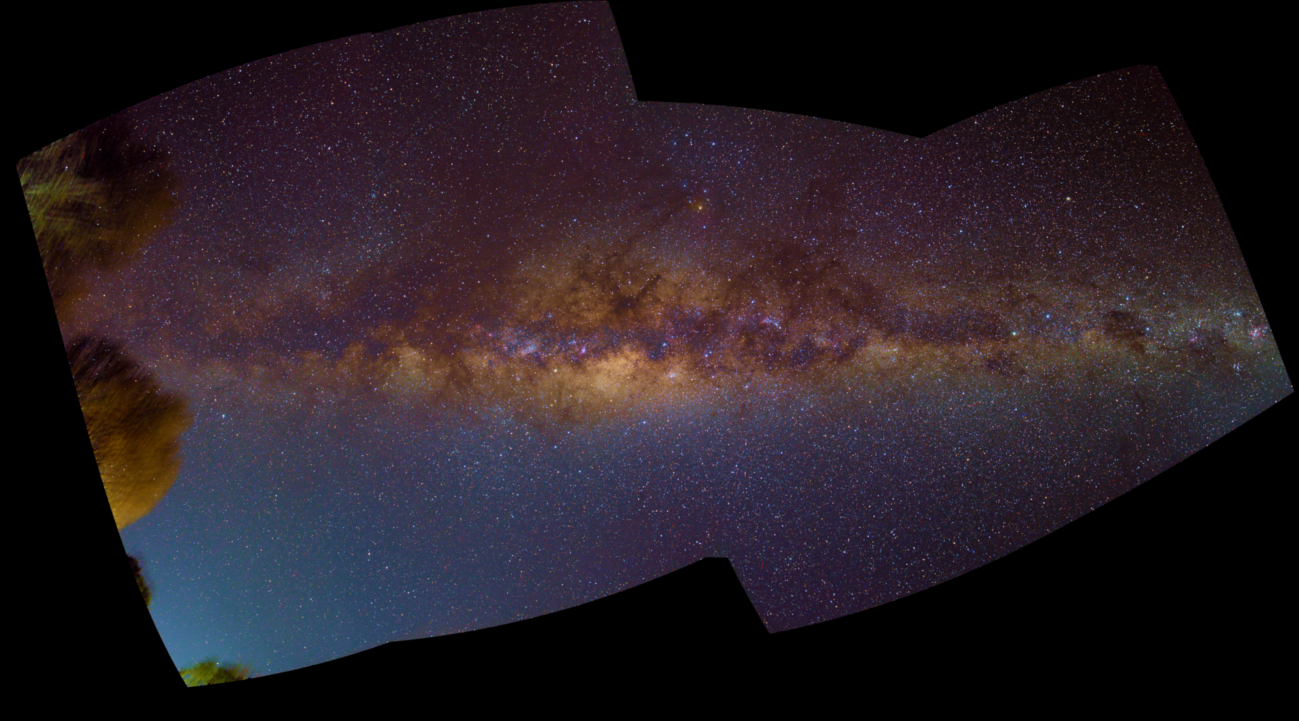
You will need the Images.jl package installed to load formats like PNG. Once the RGB image is loaded, we can store it in an AstroImage if we'd like:
mw_ai = AstroImage(mw_png)
However, we may want to extract the RGB channels first. We can do this using Images.channelview.
Images.channelview returns a view into the RGB data as a 3 × X × Y dimension cube. Unfortunately, we will have to permute the dimensions slightly.
using Images
mw_png = load("mw-crop2-small.png")
mw_chan_view = channelview(mw_png)
mw_rgb_cube = AstroImage(
    permutedims(mw_chan_view, (3, 2, 1))[:,end:-1:begin,:],
    # Optional:
    (X=:, Y=:, Spec=[:R,:G,:B])
)
╭────────────────────────────────╮
│ 2596×1440×3 AstroImage{N0f8,3} │
├────────────────────────────────┴───────────────── dims ┐
↓ X ,
→ Y ,
↗ Spec Categorical{Symbol} [:R, :G, :B] ReverseOrdered
└────────────────────────────────────────────────────────┘
[:, :, 1]
0.0 0.0 0.0 0.0 0.0 0.0 0.0 0.0 … 0.0 0.0 0.0 0.0 0.0 0.0 0.0
0.0 0.0 0.0 0.0 0.0 0.0 0.0 0.0 0.0 0.0 0.0 0.0 0.0 0.0 0.0
0.0 0.0 0.0 0.0 0.0 0.0 0.0 0.0 0.0 0.0 0.0 0.0 0.0 0.0 0.0
0.0 0.0 0.0 0.0 0.0 0.0 0.0 0.0 0.0 0.0 0.0 0.0 0.0 0.0 0.0
0.0 0.0 0.0 0.0 0.0 0.0 0.0 0.0 0.0 0.0 0.0 0.0 0.0 0.0 0.0
⋮ ⋮ ⋱ ⋮ ⋮
0.0 0.0 0.0 0.0 0.0 0.0 0.0 0.0 0.0 0.0 0.0 0.0 0.0 0.0 0.0
0.0 0.0 0.0 0.0 0.0 0.0 0.0 0.0 0.0 0.0 0.0 0.0 0.0 0.0 0.0
0.0 0.0 0.0 0.0 0.0 0.0 0.0 0.0 0.0 0.0 0.0 0.0 0.0 0.0 0.0
0.0 0.0 0.0 0.0 0.0 0.0 0.0 0.0 0.0 0.0 0.0 0.0 0.0 0.0 0.0Here we chose to mark the third axis as a spectral axis with keys :R, :G, and :B.
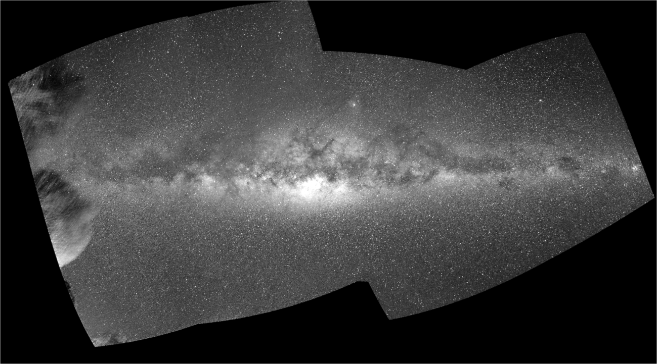
We can now visualize each channel:
mw_rgb_cube[Spec=At(:R)] # Or just: mw_rgb_cube[:,:,1]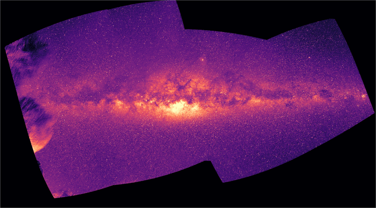
imview(
    mw_rgb_cube[Spec=At(:R)],
    cmap=nothing # Grayscale mode
)
using Plots
implot(mw_rgb_cube[Spec=At(:B)])