Plot Landsat 8 images
The data used in this example is the band 4 (red channel) of a Landsat 8 scene. Those are relatively big images (~116 MB) so we will download it first and take that into account when the results of the commands bellow do not show instantly.
I = gmtread("/vsicurl/http://landsat-pds.s3.amazonaws.com/c1/L8/037/034/LC08_L1TP_037034_20160712_20170221_01_T1/LC08_L1TP_037034_20160712_20170221_01_T1_B4.TIF");and have a look at what we got
imshow(I)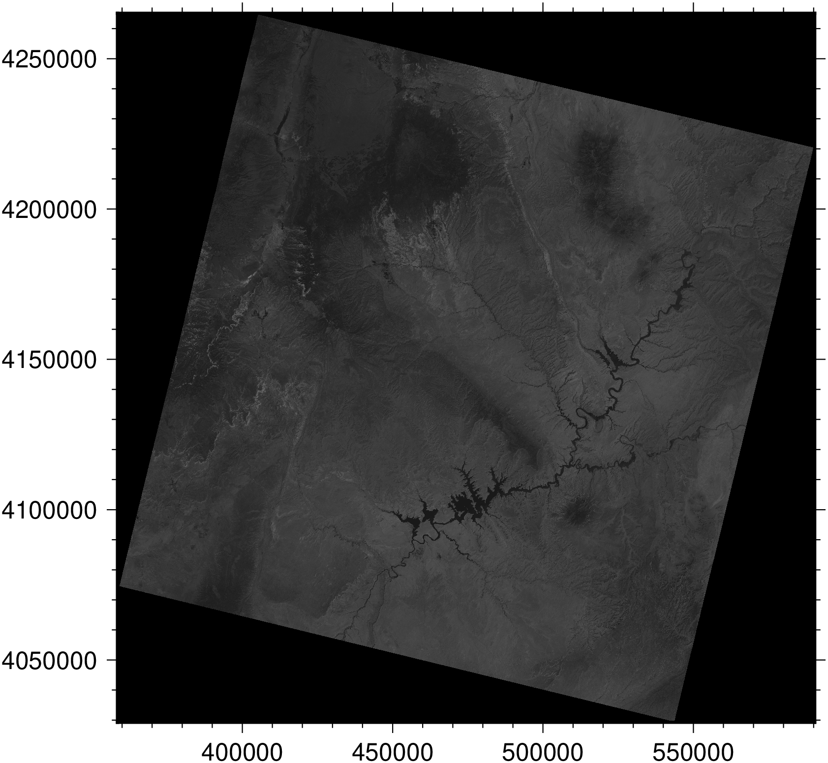
Ah, nice ... but it's so dark that we can't really see much!
Well that is true and has one explanation. Modern satellite data is acquired with sensors of 12 bits or more but the data is stored in variables with 16 bits. This means that many of those data bits will not be used. But on screens we are limited to 8 bits per channel so we must scale the full 16 bits range [0 65535] to the [0 255] interval and in this process we tend to have much more dark pixels.
To see this better, let's look at the image's histogram.
histogram(I, auto=true, bin=2, show=true)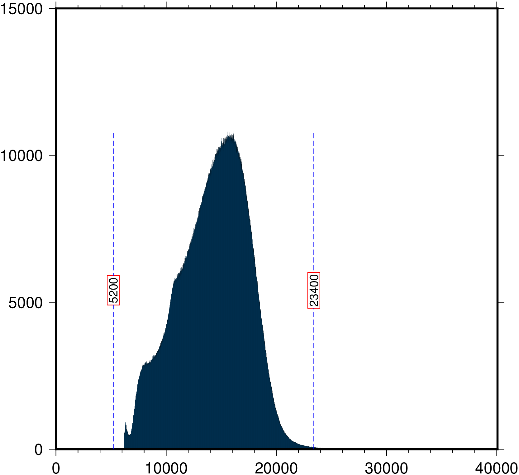
We have used here the option auto=true that will try to guess where the data in histogram plot starts and ~ ends. It did behave well and we will use those numbers to do an operation that is called histogram stretch that consists in picking only part of the histogram and stretch it to [0 255]. And while at it we van visually observe that the limit [6000 24000] seems slightly better than the automatic one. Note that in fact we have data to the 40000 DN (Digital Number) but they are very few and at the end we must choose a balance to show almos all DNs and not making the image too dark. Reducing the higher value to 23400 would have made the image sligthy lighter.
imshow(I, stretch=[6000 25000])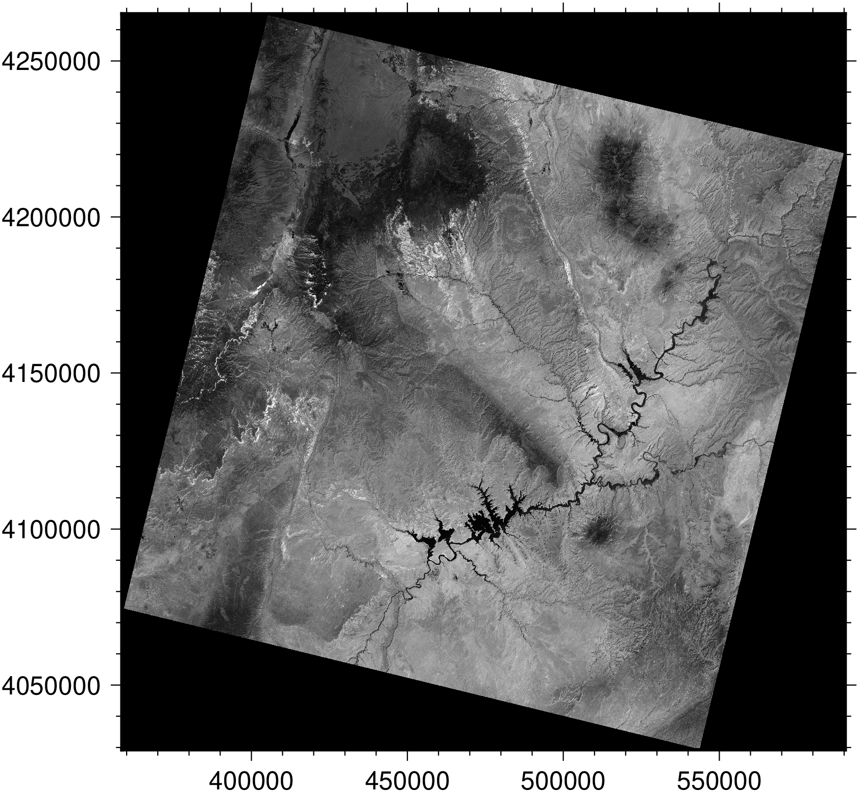
Download a Pluto Notebook here