Contourf examples

GMT does not actually have a contourf module like Matlab for example, but we can obtain the same result using grdview, grdcontour and pscontour. However, to make things the Julia wrapper wrapped up a module called contourf that makes it really easy to use. To show how it works let's start by creating an example grid and a CPT.

G = GMT.peaks();

C = makecpt(T=(-7,9,2));

Now if we pass those two to the contourf module we get an annotated plot where the annotations come from the color CPT.

contourf(G, C, show=true)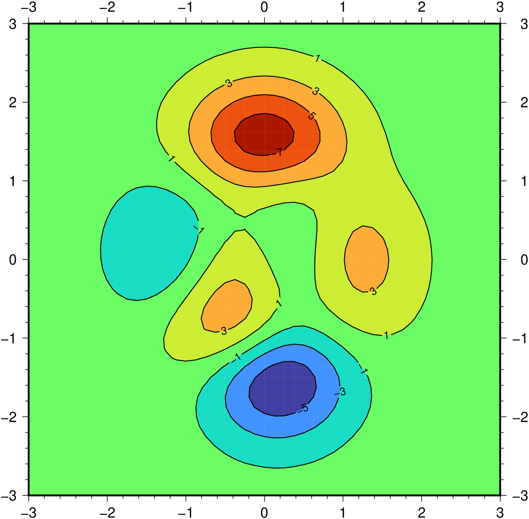

If we want to just draw some contours and not annotate them, we pass an array with the contours to be drawn.

contourf(G, C, contour=[-2, 0, 2, 5], show=true)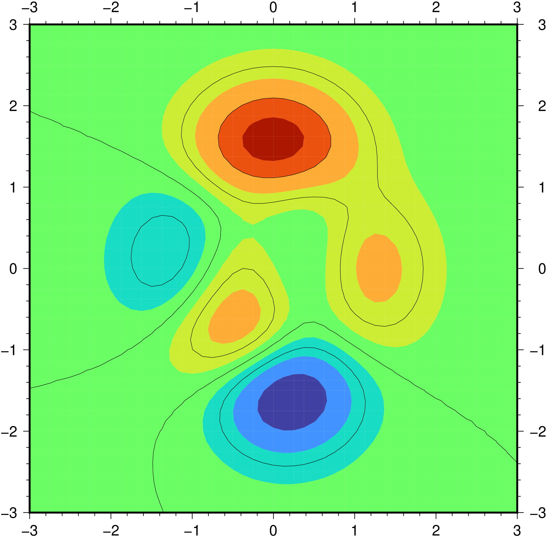

What if one has an x,y,z file instead of a grid?

That is also simple, let's simulate it with synthetic data.

d = [0 2 5; 1 4 5; 2 0.5 5; 3 3 9; 4 4.5 5; 4.2 1.2 5; 6 3 1; 8 1 5; 9 4.5 5];

contourf(d, limits=(-0.5,9.5,0,5), pen=0.25, labels=(line=(:min,:max),), show=1)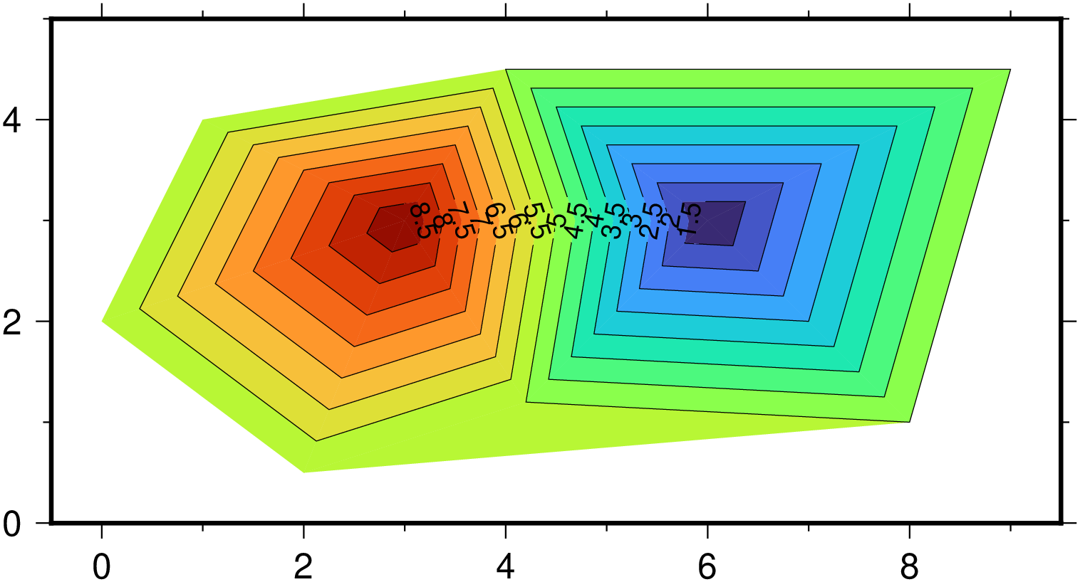

In the above since we did not specify a CPT the program picked the GMT's default one. But if we want use another one it's only a question of creating and passed it in.

cpt = makecpt(range=(0,10,1), cmap=:batlow);
contourf(d, contours=cpt, limits=(-0.5,9.5,0,5), pen=0.25, labels=(line=(:min,:max),), show=true)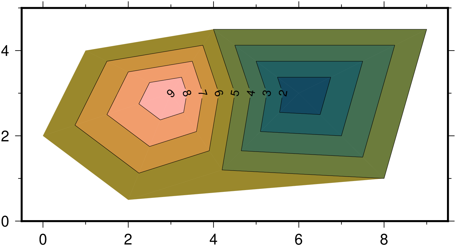

Download a Pluto Notebook here