Other Packages:
So you know what you're doing. You want to compare some basic methods available in ChemometricsTools.jl to some new stuff. Stuff that is catered to your problem - maybe stuff no one has seen before. Great! The nice thing about Julia is, packages tend to work with one another without additional effort. So we can use ChemometricsTools, and other packages to do these kinds of explorations with minimal effort. To demonstrate this I made a little tutorial using Turing.jl and ChemometricsData.jl.
This page provides a very basic, and incomplete analysis of some well known Bayesian regression methods on publicly accessible chemical data. The main goal is to show some of the Julia ecosystem working together but also to mess around with some data. This is maybe more of a survey, and me playing with Bayesian methods than anything else.
Lets load in some data
using Turing, StatsPlots, Plots, Statistics
using DataFrames, ChemometricsData, ChemometricsTools

println( ChemometricsData.search("corn") )
corn_data = ChemometricsData.load("Cargill_Corn")
X = Matrix(corn_data["m5_spectra.csv"])

xaxis = 1100:2:2498#nm

plot( X', title = "Cargill Corn M5 Spec", xlab = "Wavelength (nm)", ylab = "Absorbance", legend = false,
        xticks = (1:50:length(xaxis), xaxis[1:50:end]) )
Great out data is loaded, lets grab our property values,
Y = corn_data["property_values.csv"][!,:Moisture]Now let's split the data into a calibration set and a validation set. While we're at it, lets center and scale our X and Y values using ChemometricsTools.jl's convenience functions. We'll also down-sample our wavelength axis by a factor of 10 so our sampling goes much more quickly.
X_processed = X[:, 1:10:end]
train, test = 1:35, 36:80
X_train, X_test = X_processed[train,:], X_processed[test,:]
x_scaler = CenterScale( X_train )
X_train, X_test = x_scaler(X_train), x_scaler(X_test)

Y_train, Y_test = Y[train,:], Y[test,:]
y_scaler = CenterScale( Y_train )
Y_train, Y_test = y_scaler(Y_train ), y_scaler(Y_test )
Great now our data has been preprocessed. For fun let's try some Bayesian regression methods using the Turing.jl Pobabilistic Programming Language. On the menu for today is: Linear, Ridge, LASSO, Horseshoe, Spike-Slab, and Finnish Horseshoe regressions.
# Bayesian linear regression.
@model function lin_reg(X, y)
    obs,vars = size(X)
    α       ~ Normal(0, sqrt(3))
    β       ~ MvNormal(vars, sqrt(10))
    σ       ~ truncated( Cauchy(0., 10.0), 0, Inf)
    y       ~ MvNormal( ( X * β ) .+ α, sqrt(σ))
end

#Okay it's not ridge regression it's a cauchy prior, but that's more fun.
@model function ridge_reg(X, y)
    obs,vars = size(X)
    α       ~ Normal(0, sqrt(3))
    c       ~ truncated( Cauchy(0., 10.0), 0, Inf)
    β       ~ MvNormal( vars, c )
    σ       ~ truncated( Cauchy(0., 10.0), 0, Inf)
    y       ~ MvNormal( (X * β) .+ α, sqrt(σ))
end

"""
Not a true LASSO - but, a Laplace prior regression method. Why not?
"""
@model function LASSO_reg(X, y)
    obs,vars = size(X)
    α       ~ Normal(0, sqrt(3))
    c       ~ truncated( Cauchy(0., 100.0), 1e-6, Inf)
    β       ~ filldist( Laplace(0., c), vars)
    σ       ~ truncated( Normal(0., sqrt(3)), 1e-6, Inf)
    y       ~ MvNormal( (X * β) .+ α, sqrt(σ) )
end

"""
Code is based on the description in the following paper:
Handling Sparsity via the Horseshoe. Carlos M. Carvalho, Nicholas G. Polson, James G. Scott. 2009 Proceedings of the Twelfth International Conference on Artificial Intelligence and Statistics.
http://proceedings.mlr.press/v5/carvalho09a/carvalho09a.pdf
"""
@model function horseshoe_reg(X, y, τ0 = 1.0)
    obs,vars = size(X)
    σ       ~ truncated( Normal(0., 10.0), 0, Inf)
    λ       ~ filldist( truncated( Cauchy(0, 1),0,Inf), vars )
    τ       ~ truncated( Cauchy(0, τ0),0,Inf)
    β       ~ MvNormal(zeros(vars), λ .* τ)
    α       ~ Normal( 0, sqrt(3) )
    y       ~ MvNormal(X * β .+ α, σ)
end

"""
The code for the Finnish Horseshoe Regression is a port from PyMC3 to Turing.jl
Code and explanations can be found at the following link
https://betanalpha.github.io/assets/case_studies/bayes_sparse_regression.html (Michael Betancourt, 2018)
"""
@model function finnish_horseshoe_reg(  X, y;
                                        m0 = 3,        # Expected number of large slopes
                                        slab_scale = 2, # Scale for large slopes
                                        slab_df = 30)    # Effective degrees of freedom for large slopes
    ltz(x) = (x < 0) ? 0 : x
    obs,vars = size(X)
    M, N = obs, vars
    slab_scale2 = slab_scale^2
    half_slab_dof = 0.5 * slab_df
    σ       ~ truncated( Normal( 0, sqrt(3) ), 1e-6, Inf)
    c2      ~ truncated( InverseGamma( half_slab_dof, slab_scale2 * half_slab_dof),0,Inf)
    lambda  ~ filldist( truncated( Cauchy(0, 1), 0, Inf), vars )
    τ       ~ Cauchy( 0, ( ( m0 / (M - m0) ) * ( σ / sqrt(N) ) ) + 1e-6 )
    lambda_tilde = (sqrt( c2 ) .* lambda.^2) ./ sqrt.(c2 .+ (τ .* lambda) .^ 2)
    lambda_tilde = ltz.(lambda_tilde)
    β       ~ MvNormal( τ * lambda_tilde )
    α       ~ Normal( 0, sqrt(3) )
    y       ~ MvNormal( (X * β) .+ α, repeat([σ], obs) )
end


"""
Believe the code for spike-slab regression was written based on:
Spike and slab variable selection: Frequentist and Bayesian strategies. Hemant Ishwaran and J. Sunil Rao. Annals of Statistics. Volume 33, Number 2 (2005), 730-773.
"""
@model function spike_slab_reg(X, y, slabwidth, selection_rate = 0.25)
    csq = slabwidth^2
    obs,vars = size(X)
    λ       ~ filldist( Bernoulli( selection_rate ), vars )
    β       ~ MvNormal( λ .* csq )
    σ       ~ truncated( Cauchy(0., 10.0), 0, Inf)
    α       ~ Normal( 0, sqrt(3) )
    μ       = X * β .+ α
    y       ~ MvNormal(μ, σ)
end
Because we've chosen a pretty generic convention for our model parameters, IE: β are the coefficients and α are the bias terms, we can create a generic prediction function. Note: we allow, the user to discard some samples via burnin, and we return prediction intervals based on quantiles of "significance".
function prediction(chain, x; burnin = 1, significance = 0.05)
    p = get_params(chain[burnin:end,:,:])
    weight = reduce(hcat, p.β )
    intercept = p.α
    targets = intercept' .+ (x * weight')
    levels = [significance/2., 0.5, 1. - significance/2]
    qs = map( q -> quantile.(eachrow(targets), q), levels)
    extremes = (-3,3)
    #extrema( vcat( qs[2] .- qs[1], qs[2].+ qs[3]) )#Plot limits
    return (lower = qs[1], middle = qs[2], upper = qs[3], extremes = extremes)
end

ErrBounds(x) = ( res.middle - res.lower, res.upper - res.middle)
And now we'll begin sampling. Headsup - this will take a while.
lin_model   = lin_reg(               X_train, Y_train[:] )
rr_model    = ridge_reg(             X_train, Y_train[:] )
lr_model    = LASSO_reg(             X_train, Y_train[:] )

lin_chain = sample(lin_model, NUTS(0.999), 2_500)
rr_chain = sample(rr_model,  NUTS(0.999), 2_500)
lr_chain = sample(lr_model,  NUTS(0.999), 3_000)

hr_model    = horseshoe_reg(         X_train, Y_train[:] )
ss_model    = spike_slab_reg(        X_train, Y_train[:],  1.0, 0.3 )
fhs_model   = finnish_horseshoe_reg( X_train, Y_train[:];
                                    m0 = 4,
                                    slab_scale = 3,
                                    slab_df = 29 )

hr_chain    = sample(   hr_model,   NUTS(0.999), 2_500 )
ss_chain    = sample(   ss_model,   PG(300), 4_250 )
fhs_chain   = sample(   fhs_model,  NUTS(0.999), 2_500 )
Whew, that was a doozy, but now that it's done we can start to look at our regression coefficients. Below is an example of how we might go about doing this for one of the regression methods, but I'll spare you the plot code,
p = get_params( lin_chain[1100:end,:,:] )
lin_weight = mean( reduce(hcat, p.β ), dims = 1 )
plot( (lin_weight)', legend = false, title = "Linear Regression", xticks = newxticks );
After a lot of plot code we should see something like the following,
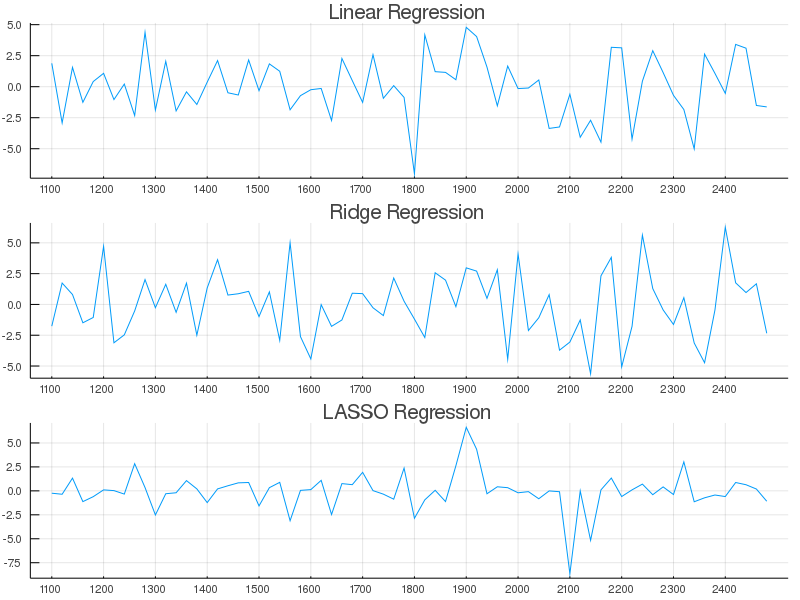
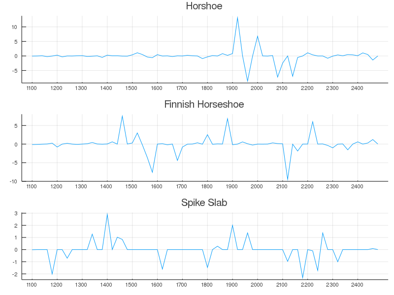
What's interesting to note here is that, as described in the literature, Bayesian LASSO does not perform like classical LASSO <sup>1</sup>. It didn't introduce true sparsity in the coefficients, but it did selectively give more weight to interesting regions than say bayesian OLS did. Fun. Mean-while, obvious feature selection/dimension reduction can be obtained by the Horseshoe, Finnish-Horseshoe, and Spike-slab regression approaches.
The Horseshoe regression method gave regression coefficients which had large weights at positions that aligned well with energies attributable to known vibrational states in water (see figure below). A small upweighting near 1500nm and much larger weights occurring around 1900-2200nm coincide somewhat well with the known absorption coefficients. Maybe not the most intuitive results, but somewhat informative nonetheless.
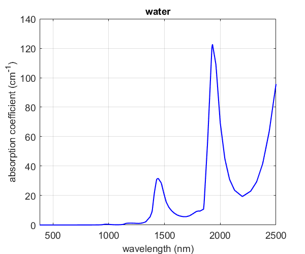
(Reference: 2)
Perhaps the results would be more clear if we did not downsample the spectra? At the end of the day, sparsity isn't everything, in NIR, the desire to have compact representations of the data is philosophically nuanced.
Sure, everyone wants a single channel in their calibration that is perfectly linear with the property of interest, has impeccable Signal-to-Noise-Ratio, and lacks interferent signal. The reality is, both analyte and interferent information in the NIR portion of the electromagnetic spectrum are extremely collinear. This makes the art of band selection, difficult. Selection of too few channels, and we may overfit chemical effects, not account for drift, or other phenomena. Too many channels, and we may have a multivariate advantage, but also, could receive sub-optimal efficacy due to scatter, noise, nonlinear contributions, decaying quantum efficiency, etc.
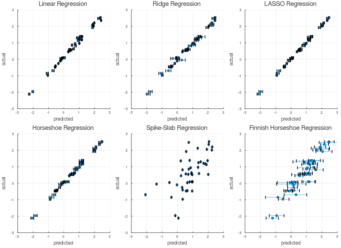
Now, we might ask ourselves, how good are these models? Sure some have interesting regression coefficients, but let's peak at some predicted vs actual plots for the training and hold out sets.
begin
    l = @layout [a b c; d e f]
    res = prediction( lin_chain, X_train; burnin = 1300 )
    a = scatter( res.middle, Y_train, xerror = ErrBounds(res), title = "Linear Regression", legend = false,
            ylim = extrema(Y_train), xlim = res.extremes, xlabel = "predicted", ylabel = "actual" )
    res = prediction( rr_chain, X_train; burnin = 1300 )
    b = scatter( res.middle, Y_train, xerror = ErrBounds(res), title = "Ridge Regression",legend = false,
            ylim = extrema(Y_train), xlim = res.extremes, xlabel = "predicted", ylabel = "actual" )
    res = prediction( lr_chain, X_train; burnin = 1600 )
    c = scatter( res.middle, Y_train, xerror = ErrBounds(res), title = "LASSO Regression",legend = false,
            ylim = extrema(Y_train), xlim = res.extremes, xlabel = "predicted", ylabel = "actual" )

    res = prediction( hr_chain, X_train; burnin = 1100 )
    d = scatter( res.middle, Y_train, xerror = ErrBounds(res), title = "Horseshoe Regression",legend = false,
            ylim = extrema(Y_train), xlim = res.extremes, xlabel = "predicted", ylabel = "actual" )
    res = prediction( ss_chain, X_train; burnin = 4000 )
    e = scatter( res.middle, Y_train, xerror = ErrBounds(res), title = "Spike-Slab Regression",legend = false,
            ylim = extrema(Y_train), xlim = res.extremes, xlabel = "predicted", ylabel = "actual" )
    res = prediction( fhs_chain, X_train; burnin = 800 )
    f = scatter( res.middle, Y_train, xerror = ErrBounds(res), title = "Finnish Horseshoe Regression", legend = false,
            ylim = extrema(Y_train), xlim = res.extremes, xlabel = "predicted", ylabel = "actual" )
    plot(a,b,c,d,e,f, layout = l, size=(1100,800))
    png("Images/train efficacy.png")
end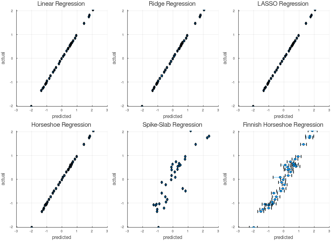
The actual vs predicted plot's provided evidence which suggested that, Finnish horseshoe regression, and Spike-Slab regression models were poor fits. In defense of these techniques, I didn't cross-validate, tune models, or do a lot of the things I'd do if this weren't a short write-up. Shoot - there could even a bug? Similarly, we'd never judge a regression by a plot or our eyes alone...
That said, the Bayesian implementations of the classical regression methods, and the horseshoe regression, appeared to perform better than the others. The posterior distributions had acceptable Rhats, and the predicted vs actual plots behaved nicely on the calibration data. Let's take a look at the hold out data,
The ability of the model to predict values matching the known properties was similar on both the calibration and validation datasets. The uncertainty of the predictions widened as we would anticipate. It appears we likely over-fit a few models. The root mean squared error tells a similar story.
chains = (      ("Linear", lin_chain, 1300),
                ("Lasso", lr_chain, 1600),
                ("Horseshoe", hr_chain, 1100),
                ("Spike-Slab", ss_chain, 4100),
                ("Finnish Horseshoe", fhs_chain, 900) )

RMSEC, RMSEP = Dict(), Dict()

for (name, chain, burnin) in chains
        cal = y_scaler( prediction( chain, X_train; burnin = burnin ).middle, inverse = true  )
        rescale =  y_scaler( Y_train, inverse = true )
        RMSEC[name] = RMSE( cal, rescale )

        val = y_scaler( prediction( chain, X_test; burnin = burnin ).middle, inverse = true)
        rescale =  y_scaler( Y_test, inverse = true )
        RMSEP[name] = RMSE( val, rescale )
end
field_df = DataFrame("Type" => [:RMSEC, :RMSEP])
out_df = vcat( DataFrame(RMSEC), DataFrame(RMSEP) )

println(hcat(field_df,out_df))
2×7 DataFrame
│ Type │ Finnish Horseshoe │ Horseshoe │ Lasso │ Linear │ Ridge │ Spike-Slab │
│ Symbol │ Float64 │ Float64 │ Float64 │ Float64 │ Float64 │ Float64 │
├────────┼───────────────────┼────────────┼────────────┼────────────┼────────────┼────────────┤
│ RMSEC │ 0.0692553 │ 0.00793535 │ 0.00299732 │ 0.00465332 │ 0.00558598 │ 0.172215 │
│ RMSEP │ 0.156203 │ 0.0324 │ 0.0208388 │ 0.0609198 │ 0.0432594 │ 0.303853 │The nonsparse and sparse methods with the lowest validation error were the LASSO and Horseshoe regressions respectively. For a frame of reference, let's consider how PLS-1 performs using the exact same pretreatments.
Err = repeat([0.0], 16);
Models = []
for Lv in 16:-1:1
    for ( i, ( Fold, HoldOut ) ) in enumerate(KFoldsValidation(10, X_train, Y_train))
        if Lv == 16
            push!( Models, PartialLeastSquares(Fold[1], Fold[2]; Factors = Lv) )
        end
        Err[Lv] += SSE( Models[i]( HoldOut[1]; Factors = Lv), HoldOut[2] )
    end
end
#scatter(Err, xlabel = "Latent Variables", ylabel = "Cumulative SSE", title = "10-Folds", labels = "SSE")
BestLV = 7
PLSR = PartialLeastSquares(X_train, Y_train; Factors = BestLV)
pls_rmsec = RMSE( y_scaler( PLSR(X_train) , inverse = true), y_scaler(Y_train, inverse = true) )
pls_rmsep = RMSE( y_scaler( PLSR(X_test) , inverse = true), y_scaler(Y_test, inverse = true)  )

field_df = DataFrame("PLS-1" => [pls_rmsec, pls_rmsep])
println(hcat(out_df,field_df))
2×8 DataFrame
│ Row │ Type │ Finnish Horseshoe │ Horseshoe │ Lasso │ Linear │ Ridge │ Spike-Slab │ PLS-1 │
│ │ Symbol │ Float64 │ Float64 │ Float64 │ Float64 │ Float64 │ Float64 │ Float64 │
├─────┼────────┼───────────────────┼────────────┼────────────┼────────────┼────────────┼────────────┼───────────┤
│ 1 │ RMSEC │ 0.0692553 │ 0.00793535 │ 0.00299732 │ 0.00465332 │ 0.00558598 │ 0.172215 │ 0.0288213 │
│ 2 │ RMSEP │ 0.156203 │ 0.0324 │ 0.0208388 │ 0.0609198 │ 0.0432594 │ 0.303853 │ 0.0430593 │In this case, Bayesian ridge regression afforded a predictive error that was similar in magnitude to PLS-1. This isn't an unusual result, but, it seems convenient. In many instances we see Ridge regression performing about as well as PLS-1. The fun part here is, we didn't have to search for a regularization hyperparameter, rely on say the spectral norm of the design matrix, or empirically find some number of latent factors. When we changed the problem statement to be based on distributions and not scalar parameters, the Monte Carlo optimization optimized this distribution for us.
Worth noting, the Bayesian approach also provided us with uncertainty estimates - for free. Okay, not for free, the computer definitely calculated them, but we didn't need to provide analytic expressions, propagate error over a compute graph, etc. This is a serious advantage of Bayesian modelling methods. The discussion of calculating prediction intervals for advanced regression methods can be extremely technical, and in some cases, world experts are still scratching their heads...
Conclusions
As you can see, the Julia ecosystem is very flexible. We are able to load data from ChemometricsData.jl, do preprocessing via ChemometricsTools.jl, build some compute heavy models in Turing.jl, perform a little post analysis with Statistics.jl, ChemometricsTools.jl, and organize data with DataFrames.jl. All without much trouble whatsoever.
Which model would I choose? Personally I'd choose none of these, I'd spend more time tuning the Turing models and giving each approach a fair chance. Seeing what I could learn from each, and then combining that knowledge into a final model. I'd also introduce more metrics, statistical tests, and examine more plots than what is shown here. Unfortunately, life is rough, and I don't have time to do that right now. But - to escape some caveats - if I had to chose one, say a deadline was coming up, I would likely choose the horseshoe regression. This method afforded model weights that although not statistically validated, matched an empirical result "okay". That's better than nothing!
References
- Trevor Park & George Casella (2008) The Bayesian Lasso, Journal of the American Statistical Association, 103:482, 681-686, DOI: 10.1198/016214508000000337)
- K.F. Palmer and D. Williams, "Optical Properties of water in the near infrared," Journal of the Optical Society of America, V.64, pp. 1107-1110, August, 1974.