CSP

The Common Spatial Pattern (CSP) are filters obtained by generalized eigenvalue-eigenvector decomposition. They corresponds to the situation $m=1$ (one dataset) and $k=2$ (two observation). The goal of a CSP filter is to maximize a variance ratio. Let $(X_1, X_2)$ be $(n⋅t_1, n⋅t_2)$ data matrices, where $n$ is their number of variables and $(t_1, t_2)$ their number of samples. Let $(C_1, C_2)$ be the $n⋅n$ covariance matrices of data matrices $(X_1, X_2)$ and $C=C_1+C_2$. The CSP consists in the joint diagonalization of $C$ and $C_1$ or, equivalently, of $C$ and $C_2$ (Fukunaga, 1990, p. 31-33 🎓). The joint diagonalizer $B$ is scaled such as to verify (see scale and permutation)

$\left \{ \begin{array}{rl}B^TCB=I\\B^TC_1B=Λ\\B^TC_2B=I-Λ \end{array} \right.$, $\hspace{1cm}$ [csp.1]

That is to say, $λ_1≥\ldots≥λ_n$ are the diagonal elements of $B^TC_1B$ and $1-λ_1≤\ldots≤1-λ_n$ the diagonal elements of $B^TC_2B$. The CSP maximizes the ratio between the variance of the corresponding components of transformed processes $B^TX_1$ and $B^TX_2$, constraining their sum to unity. The ratio is ordered by descending order such as

$σ=[λ_1/(1-λ_1)≥\ldots≥λ_n/(1-λ_n)]$, $\hspace{1cm}$ [csp.2]

The CSP has two use cases, which can be selected using the selMeth optional keyword argument of its constructors:

• a) Separating two classes. In this case $C_1$ and $C_2$ are covariance matrices of two distinct classes. The constructors will retain a filter with form $\widetilde{B}=[B_1 B_2]$, where we have defined partitions $B=[B_1 B_0 B_2]$. $B_1$ and $B_2$ are the first $p_1$ and last $p_2$ vectors of $B$ corresponding to high and low values of the variance ratio [csp.2], that is, explaining variance that is useful for separating the classes, while $B_0$ corresponds to components corresponding to variance ratios close to $1$, meaning that are not useful for separating the classes. The subspace dimension in this use case will be given by $p=p_1+p_2$. Notice that in Diagonalizations.jl we allow $p_1≠p_2$.
• b) Enhance the signal-to-noise ratio. In this case $C_1$ and $C_2$ are covariance matrices of the 'signal' and of the 'noise', respectively. The constructors will retain a filter $\widetilde{B}=[b_1 \ldots b_p]$ holding the first $p$ vectors of $B$ corresponding to the highest values of the variance ratio [csp.2]. The discared $n-p$ vectors correspond to components that explains progressively more and more variance related to the noise process. In this case we have a natural landmark for selecting automatically the subspace dimension$p$, as the larger dimension whose variance ratio is greater then $1$.

In order to retrive the appropriate partitions of $B$ to construct a filter given a subspace dimension $p$, we need a way to measure the distance of the ratios [csp.2] from $1$. For this purpose we will make use of the Fisher distance adopted on the Riemannian manifold of positive definite matrices, in its scalar form, yielding

$δ_i=\textrm{log}^2(σ_i)$, for $i=[1 \ldots n]$. $\hspace{1cm}$ [csp.3]

After this transformation, extreme values of the ratio becomes high, that is, the function $δ_i$ assumes the shape of a (non-symmetric) wine cup and has a minimum close to zero.

Now let $δ_{TOT}=\sum_{i=1}^nδ_i$ be the total distance and define the explained variance of the CSP for dimension $p$ such as

$v_p=\frac{\sum_{j=1}^pδ_j}{δ_{TOT}}$, $\hspace{1cm}$ [csp.4]

where the $δ_j$'s are given by [csp.3]. Note that for use case a) described here above the accumulated sums in [csp.4] are computed after sorting the $δ_i$ values in descending order.

The $.arev$ field of CSP filter is defined as the accumulated variance ratio given by

$[v_1≤\ldots≤v_n]$, $\hspace{1cm}$ [csp.5]

where the $v_i$'s' are defined in [csp.4].

For setting the subspace dimension $p$ manually, set the eVar optional keyword argument of the CSP constructors either to an integer or to a real number (see subspace dimension). If you don't, by default $p$ is chosen (see Fig. 2)

• in use case a) as the larger dimension $p$ whose sorted $δ_p$ value [csp.3] is larger then the geometric mean of $δ$$1$. $n÷2$ is taken as upper bound.
• in use case b) as the larger dimension $p$ whose $σ_p$ value [csp.2] is larger then $1$.

In both cases the dimension corresponding to the munimum of [csp.3] is taken as an upper bound and $p$ can be equal to at most $n-1$.

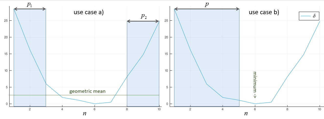Figure 2Illustration of the way CSP constrcuctors determines automatically the subspace dimension $p$ under use case a) and b). On the left, we are interested in the $p_1$ and $p_2$ vectors of $B$ associated with extremal values of the variance ratios [csp.2], which are the high values of $δ$ [csp.3] enclosed in the shaded boxes of the figure. The threshold is set to the geometric mean of $δ$. Since Diagonalizations.jl always sorts the explained variance in descending order, $\widetilde{B}$ is defined as $[b_1, b_{10}, b_9, b_2, b_8, b_3]$. On the right, we are interested in the first $p$ vectors of $B$ associated with positive values of the variance ratios [csp.2], which are the high values on the left of the minimum of $δ$ enclosed in the shaded box of the figure. The threshold is set in this case to the first value of $σ$ [csp.2] smaller then $1$, which roughly coincides with the minimum of $δ$ reported in the figure. Assuming in this example they do coincide, $\widetilde{B}$ would be defined as $[b_1 \ldots b_5]$.

Solution

The CSP solution $B$ is given by the generalized eigenvalue-eigenvector decomposition of the pair $(C, C_1)$.

A numerically preferable solution is the following two-step procedure:

1. get a whitening matrix $\hspace{0.1cm}W\hspace{0.1cm}$ such that $\hspace{0.1cm}W^TCW=I\hspace{0.1cm}$.
2. do $\hspace{0.1cm}\textrm{EVD}(W^TC_{1}W)=UΛU^{T}$

The solution is $\hspace{0.1cm}B=WU$.

Constructors

Three constructors are available (see here below). The constructed LinearFilter object holding the CSP will have fields:

.F: matrix $\widetilde{B}$ as defined above. This is just $B$ of [csp.1] if optional keyword argument simple=true is passed to the constructors (see below).

.iF: the left-inverse of .F

.D: the $p⋅p$ diagonal matrix with the elements of $Λ$ [csp.1] corresponding to the vectors of $\widetilde{B}$.

.eVar: the explained variance for the chosen value of $p$, given by the $p^{th}$ value of [csp.5]

.ev: the vector holding all $n$ generalized eigenvalues, i.e., the diagonal elements of matrix $Λ$ [csp.1]. Notice that if selMeth=:extremal these elements are sorted differently than in .D and their position do not correspond to the vectors of .F.

.arev: the accumulated regularized eigenvalues, defined in [csp.5].