NodeConstructor Theory

The NodeConstructor has the goal to convert the physical system, here the grid, into a mathematical model. This mathematical model can then be used to simulate the behavior of the network. This notebook addresses the following points:

• Introduction to the NodeConstructor

• Representation of the physical grid

• Building of the state-space matrices

Introduction

The NodeConstructor is part of the enviroment (see graphic). Its function is to create the mathematical model of the grid to be simulated. The inputs for the NodeConstructor are the specifications of the grid, which will be discussed in more detail subsequently. Within the NodeConstructor, an ordinary differential equation (ODE) system is created based on the underlying physical models and properties of the individual components. Based on this ODE system, the necessary matrices can be extracted.

In the following, we will discuss how the mathematical model of an electrical power grid can be generated using the NodeConstructor.

Modelling a physical grid

The following graphic shows a simple example grid:

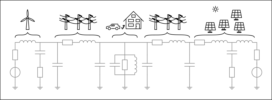
Two sources (wind turbine on the left and PV arrays on the right), as well as a load (exemplary of a household which is composed of various objects) can be seen in this. In addition, the sources are connected to the load via cables. For the sources, we assume that the voltage is provided by a DC link, so we can assume that the voltage can be modeled by a voltage source and a filter. Loads are divided into active loads, which, based on an internal function, can take power from the network, and passive loads, which are described by their resistive, capacitive and/or inductive components and thus dissipate a certain power. Cable modeling relies on the Pi equivalent circuit like depicted in the fiure below.

If you abstract the above figure and insert the respective components according to the description, you get the following single-phase circuit:

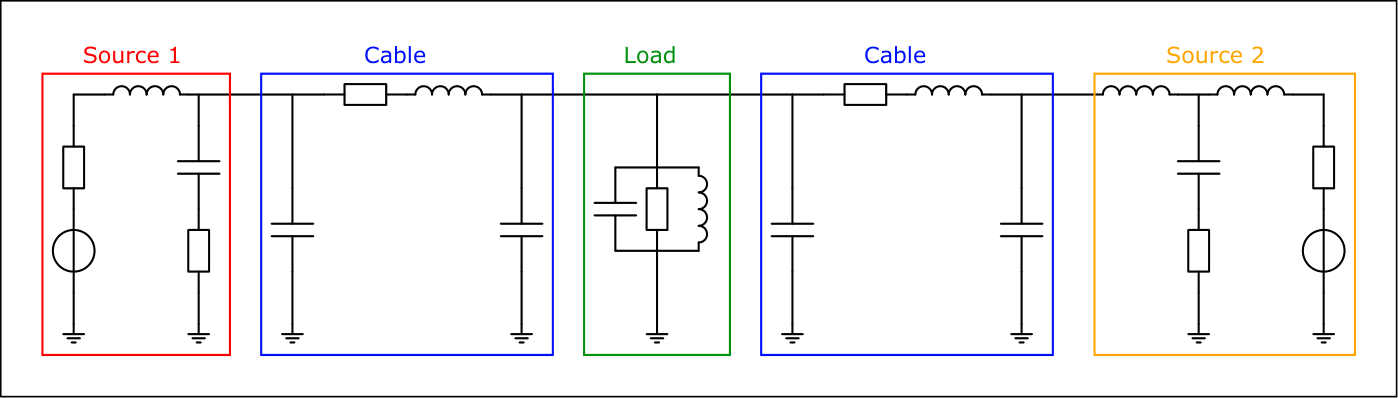
With the help of this example, we will now discuss the derivation of a mathematical model and what information the NodeConstructor will later need to generate this model automatically.

Fundamentals of electrical engineering

If we annotate the above equivalent circuit, we get the following representation:

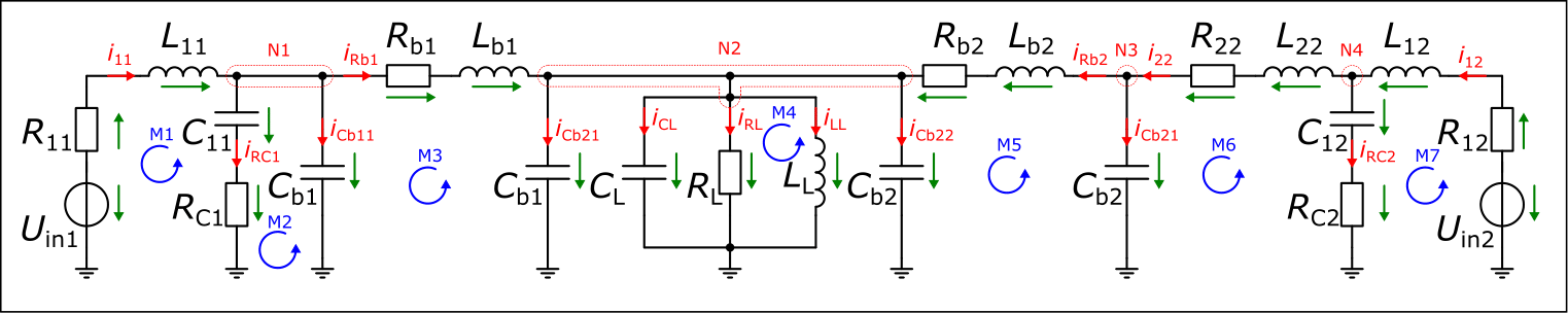
In this, the components are annotated and the currents are noted with the technical flow direction. For the sake of clarity, the voltages are only indicated by green arrows, but have the same name as the corresponding component to which they are applied.

Based on the components within the equivalent circuit diagram, we can now construct the differential equations. Togehter with Kirchhoff's laws

\[\begin{align} \sum_k^n i_k(t) &= 0,\\ \sum_k^n u_n(t) &= 0 \end{align}\]

and the component equations

\[\begin{align} u(t) &= R i(t),\\ i(t) &= C\dot u(t),\\ u(t) &= L\dot i(t). \end{align}\]

This gives the following equation system:

\[\begin{align} \text{M1:}\;& 0 = u_{in1} - u_{R11} - u_{L11} - u_{C11} - u_{RC1}, \tag{1}\\ \text{M2:}\;& 0 = u_{C11} + u_{RC1} - u_{Cb11},\tag{2}\\ \text{M3:}\;& 0 = u_{Cb11} - u_{Rb1} - u_{Lb1} - u_{Cb21},\tag{3}\\ \text{M4:}\;& 0 = u_{RL} - u_{LL}, \tag{4}\\ \text{M5:}\;& 0 = u_{Cb22} + u_{Rb2} + u_{Lb2} - u_{Cb12}, \tag{5}\\ \text{M6:}\;& 0 = u_{Cb12} + u_{R22} + u_{L22} - u_{C12} - u_{RC2}, \tag{6}\\ \text{M7:}\;& 0 = u_{RC2} + u_{C12} + u_{L12} + u_{R12} - u_{in2}, \tag{7}\\ \text{N1:}\;& 0 = i_{11} - i_{RC1} - i_{Cb11} - i_{Rb1}, \tag{8}\\ \text{N2:}\;& 0 = i_{Rb1} - i_{Cb21} - i_{CL} - i_{RL} - i_{LL} - i_{Cb22} + i_{Rb2}, \tag{9}\\ \text{N3:}\;& 0 = i_{22} - i_{Rb2} - i_{Cb21}, \tag{10}\\ \text{N4:}\;& 0 = i_{12} - i_{RC2} - i_{22}. \tag{11} \end{align}\]

For the sake of clarity, the time dependencies are omitted here. For node 2 the connected capacitances are summed up, because there are several capacitors connected in parallel, e.g.:

\[\begin{equation} C_{SL} = C_{b1} + C_L + C_{b2} \end{equation}\]

We then call this capacitor $C_{SL}$ through which the current $i_{CSL}$ flows and the voltage $u_{CSL}$ is applied. Now we insert the component equations into the equations (1) to (11) and rearrange them, so that an ODE system is obtained:

\[\begin{align} \dot i_{11} &= \frac{1}{L_{11}} \left( u_{in1} - R_{11} i_{11} - R_{RC1} i_{RC1} - u_{C12} \right), \\ \dot u_{C11} &= \frac{1}{C_{11}R_{C11}} \left(u_{Cb11} - u_{RC1} \right), \\ \dot i_{Rb1} &= \frac{1}{L_{b1}} \left( u_{Cb11} - i_{Rb1} R_{b1} \right),\\ \dot i_{LL} &= \frac{1}{L_{L}} u_{CL}\\ \dot i_{Rb2} &= \frac{1}{L_{b2}} \left( u_{Cb12} - i_{Rb2} R_{b2} - u_{Cb22}\right),\\ \dot i_{22} &= \frac{1}{L_{22}} \left( u_{C12} - i_{22} (R_{C2}+R_{22}) - R_{RC1} i_{RC2} - u_{Cb12} \right), \\ \dot i_{12} &= \frac{1}{L_{12}} \left( u_{in2} - i_{12} (R_{12} + R_{RC1}) - R_{RC1} i_{C1} - u_{C12} \right), \\ \dot u_{Cb11} &= \frac{1}{C_{b1}} \left(i_{11} - i_{Rb1} - \frac{1}{R_{C1}} u_{Cb11} + \frac{1}{R_{C1}} u_{C11}\right),\\ \dot u_{CSL} &= \frac{1}{C_{SL}} \left( i_{Rb1} + i_{Rb2} - \frac{1}{R_{L}} u_{CSL} - i_{LL} \right),\\ \dot u_{Cb12} &= \frac{1}{C_{b2}} \left(i_{22} - i_{Rb2}\right),\\ \dot u_{C12} &= \frac{1}{C_{12}} \left(i_{12} - i_{22}\right).\\ \end{align}\]

These differential equations describe the system completely and could be solved for exampled using numerical solvers like Forward Euler or Runge-Kutta.

Forming the system matrices from the ODEs

The differential equations found are now to be converted into the common state-space representation:

\[\begin{align} \dot{\vec{x}}(t) &= \mathbf{A} \vec{x}(t) + \mathbf{B} \vec{u}(t)\\ \vec{y}(t) &= \mathbf{C} \vec{x}(t) + \mathbf{D} \vec{u}(t) \end{align}\]

Since we are interested in how our grid evolves over time, the first equation is most relevant to our application. $x(t)$ describes in general the state vector, $\dot x(t)$ the changes of this state vector. The change of the system is described on the one hand by the system dynamics, which is expressed by the matrix $\mathbf{A}$ and on the other hand by the input signals $u(t)$ acting on the system combined with the matrix $\mathbf{B}$.

For our example, we can find the following state vector:

\[\begin{equation} \vec{x}(t) = \begin{pmatrix} i_{11} & u_{C11} & u_{Cb11} & i_{12} & u_{C12} & i_{22} & u_{Cb12} & i_{Rb1} & i_{Rb2} & u_{CSL} & i_{LL} \end{pmatrix}^\top \end{equation}\]

and the following input vector:

\[\begin{equation} \vec{u}(t) = \begin{pmatrix} u_{in1} & u_{in2} \end{pmatrix}^\top. \end{equation}\]

It should be noted that the order of the states here is first sources, then cables and finally the loads.

This leads for the investigated example to the following matrices:

\[\begin{equation} \mathbf{A} = \begin{pmatrix} -\frac{R_{11}}{L_{11}} & 0 & -\frac{1}{L_{11}} & 0 & 0 & 0 & 0 & 0 & 0 & 0 & 0\\ 0 & -\frac{1}{C_{11} R_{C1}} & \frac{1}{C_{11} R_{C1}} & 0 & 0 & 0 & 0 & 0 & 0 & 0 & 0\\ \frac{1}{C_{b1}} & \frac{1}{C_{b1} R_{C1}} & -\frac{1}{C_{b1} R_{C1}} & 0 & 0 & 0 & 0 & -\frac{1}{C_{b1}} & 0 & 0 & 0\\ 0 & 0 & 0 & -\frac{R_{12} + R_{C2}}{L_{12}} & -\frac{1}{L_{12}} & \frac{R_{C2}}{L_{12}} & 0 & 0 & 0 & 0 & 0\\ 0 & 0 & 0 & \frac{1}{C_{12}} & 0 & -\frac{1}{C_{12}} & 0 & 0 & 0 & 0 & 0\\ 0 & 0 & 0 & \frac{R_{C2}}{L_{22}} & \frac{1}{L_{22}} & -\frac{R_{22} + R_{C2}}{L_{22}} & -\frac{1}{L_{22}} &0&0&0&0\\ 0 & 0 & 0 & 0 & 0 & \frac{1}{C_{b2}} & 0 & 0 & -\frac{1}{C_{b2}} & 0 & 0\\ 0 & 0 & \frac{1}{L_{b1}} & 0 & 0 & 0 & 0 & -\frac{R_{b1}}{L_{b1}} & 0 & -\frac{1}{L_{b1}} & 0\\ 0 & 0 & 0 & 0 & 0 & 0 & \frac{1}{L_{b2}} & 0 & -\frac{R_{b2}}{L_{b1}} & -\frac{1}{L_{b2}} & 0\\ 0 & 0 & 0 & 0 & 0 & 0 & 0 & \frac{1}{C_{SL}} & \frac{1}{C_{SL}} & -\frac{1}{R_{L} C_{SL}} & -\frac{1}{C_{SL}}\\ 0 & 0 & 0 & 0 & 0 & 0 & 0 & 0 & 0 & \frac{1}{L_{L}} & 0\\ \end{pmatrix} \end{equation}\]

and

\[\begin{equation} \mathbf{B} = \begin{pmatrix} \frac{1}{L_{11}} & 0 \\ 0 & 0 \\ 0 & 0 \\ 0 & \frac{1}{L_{12}} \\ 0 & 0 \\ 0 & 0 \\ 0 & 0 \\ 0 & 0 \\ 0 & 0 \\ 0 & 0 \\ 0 & 0 \\ \end{pmatrix} \end{equation}\]

Solving the ODE system

Now we will deal with the solving of the ODE. The ODE was defined above in continuous time, but since we are in a digital environment, it first has to be discretised and optain the diverence equations in discret time. Assuming ideal digital-to-analogue (D/A) and analogue-to-digital (A/D) conversion with zero-order hold capability, the following system of equations results:

\[\begin{align} \dot{\vec{x}}[k] &= \mathbf{A}_d \vec{x}[k] + \mathbf{B}_d \vec{u}[k]\\ \vec{y}[k] &= \mathbf{C}_d \vec{x}[k] + \mathbf{D}_d \vec{u}[k] \end{align}\]

Note that the matrices $\mathbf{A}_d$ and $\mathbf{B}_d$ are different from the continuous-time counterparts. Further below it will be shown how these can be discretised. There are several tools to solve the difference equation. We use the ControlSystem package (Source), to be more precise the lsim() function.

using ControlSystemsBase
using LinearAlgebra
using PlotlyJS

Next we define some the values of the components:

# Source
R = 1.1e-3
L = 70e-6
R_c = 7e-3
C = 250e-6

# Cable
C_b = 1e-4/2
L_b = 1e-4
R_b = 1e-3

# Load
R_l = 100
C_l = 1e-2
L_l = 1e-2;

Now we construct the matrices:

A = zeros((11,11))
A[1,1] = -R/L
A[1,3] = -1/L
A[2,2] = -1/(C*R_c)
A[2,3] = 1/(C*R_c)
A[3,1] = 1/C_b
A[3,2] = 1/(R_c*C_b)
A[3,3] = -1/(R_c*C_b)
A[3,8] = -1/C_b
A[4,4] = -(R+R_c)/L
A[4,5] = -1/L
A[4,6] = R_c/L
A[5,4] = 1/C
A[5,6] = -1/C
A[6,4] = R_c/L
A[6,5] = 1/L
A[6,6] = -(R+R_c)/L
A[6,7] = -1/L
A[7,6] = 1/C_b
A[7,9] = -1/C_b
A[8,3] = 1/L_b
A[8,8] = -R_b/L_b
A[8,10] = -1/L_b
A[9,7] = 1/L_b
A[9,9] = -R_b/L_b
A[9,10] = -1/L_b

C_SL = C_b + C_l + C_b

A[10,8] = 1/C_SL
A[10,9] = 1/C_SL
A[10,10] = -1/(R_l*C_SL)
A[10,11] = -1/C_SL
A[11,10] = 1/L_l;

B = zeros((11,2))

B[1,1] = 1/L
B[4,2] = 1/L;

C = Diagonal(ones(11));

D = 0;

We convert the matrices into the discrete time domain and create a discrete StateSpace object with the help of ControlSystems. This object can then represent the dynamics of the system for a given time interval using the function lsim().

ts = 1e-5
Ad = exp(A*ts)
Bd = A \ (Ad - C) * B
sys_d = StateSpace(Ad, Bd, C, D, ts);

ns = length(A[1,:]) # get num of states
ni = length(B[1,:]) # get num of inputs
t = collect(0:ts:0.1)
x0 = [0.0 for i = 1:ns]
u = [230.0 for i = 1:length(t)]
uu = [u for i = 1:ni ]
uuu = mapreduce(permutedims, vcat, uu);

To use lsim() you need defined initial states x0, a time vector t and a input signal u. In our case we apply a jump to 230 V to the system.

xout, _, _, _ = lsim(sys_d,uuu,t,x0=x0);

layout = Layout(xaxis_title="Time in µs", yaxis_title="v_C / V")
p = plot(t, xout[5,:], layout)