Exercise: Inverse Modeling with ADCME

Background

The thermal diffusivity is the measure of the ease at which the heat can pass through a material. Let $u$ be the temperature, and $\kappa$ be the thermal diffusivity. The heat transfer process is described by the Fourier's law

Here $f$ is the heat source and $\Omega$ is the domain.

To make use of the heat equation, we need additional information.

• Initial Condition: the initial temperature distribution is given $u(\mathbf{x}, 0) = u_0(\mathbf{x})$.

• Boundary Conditions: the temperature of the material is affected by what happens on the boundary. There are several possible boundary conditions. In this exercise we consider two of them:

  (1) Temperature fixed at a boundary,

  \[u(\mathbf{x}, t) = 0, \mathbf{x}\in \Gamma_D \tag{2}\]

  (2) Insulated boundary. The heat flow can be prescribed (known as the no flow boundary condition)

  \[-\kappa\frac{\partial u(\mathbf{x},t)}{\partial n} = 0, \mathbf{x}\in \Gamma_N \tag{3}\]

  Here $n$ is the outward normal vector.

  The boundaries $\Gamma_D$ and $\Gamma_N$ satisfy $\partial \Omega = \Gamma_D \cup \Gamma_N, \Gamma_D\cap \Gamma_N=\empty$.

Assume that we want to experiment with a piece of new material. The thermal diffusivity coefficient of the material is an unknown function of the space. Our goal of the experiment is to find out the thermal diffusivity coefficient. To this end, we place some sensors in the domain or on the boundary. The measurements are sparse in the sense that only the temperature from those sensors–-but nowhere else–-are collected. Namely, let the sensors be located at $\{\mathbf{x}_i\}_{i=1}^M$, then we can observe $\{\hat u(\mathbf{x}_i, t)\}_{i=1}^M$, i.e., the measurements of $\{ u(\mathbf{x}_i, t)\}_{i=1}^M$. We also assume that the boundary conditions, initial conditions and the source terms are known.

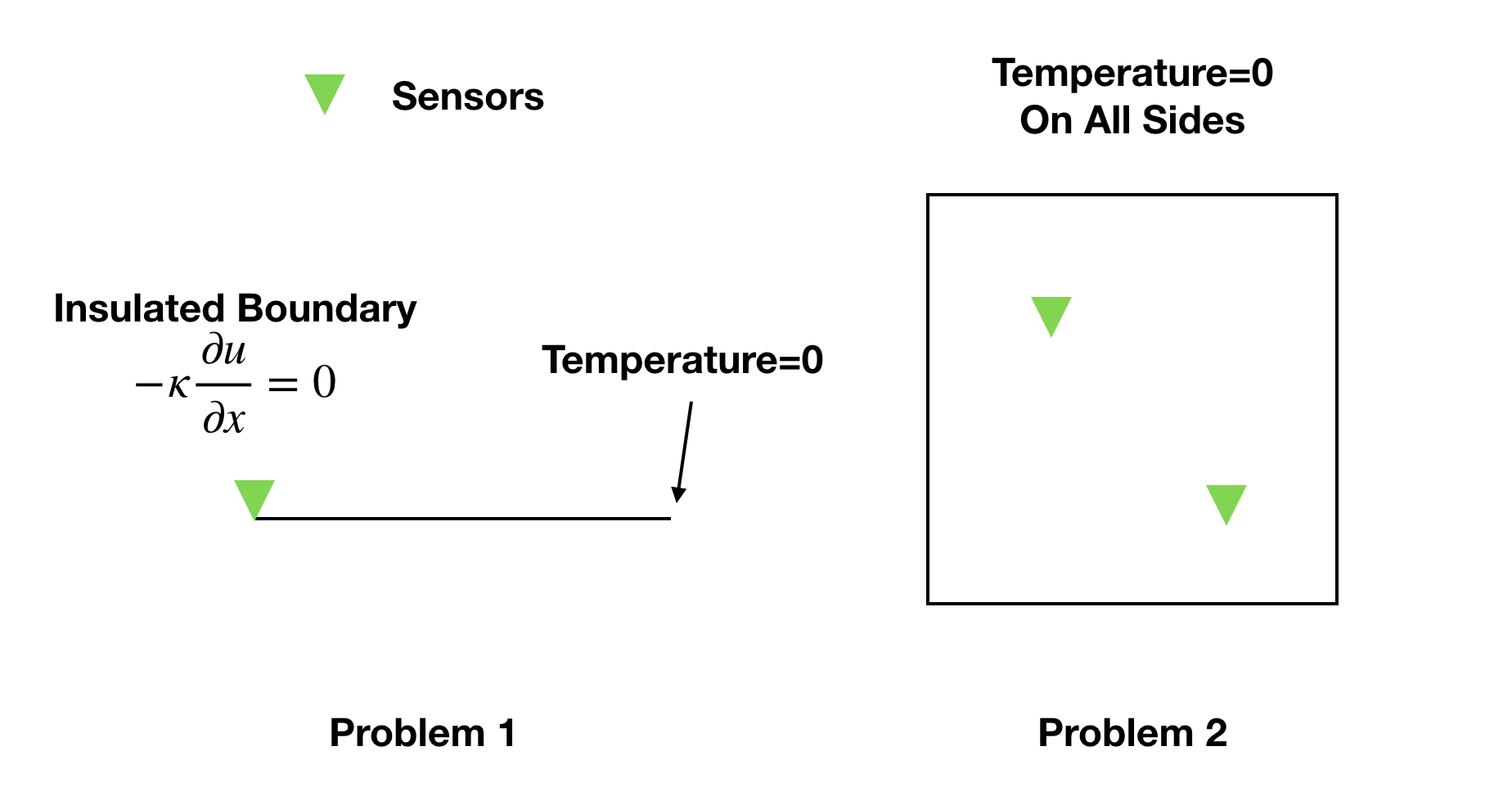
Problem 1: Parameter Inverse Problem in 1D

We first consider the simpler 1D case. In this problem the material is a rod $\Omega=[0,1]$. We consider a homogeneous (zero) fixed boundary condition on the right side, and an insulated boundary on the left side. The initial temperature is zero everywhere, i.e., $u(x, 0)=0$, $x\in [0,1]$. The source term is $f(x, t) = \exp(-10(x-0.5)^2)$, and $\kappa(x)$ is a function of space

Our task is to estimate the coefficient $a$ and $b$ in $\kappa(x)$. To this end, we place a sensor at $x=0$, and the sensor records the temperature as a time series $u_0(t)$, $t\in (0,1)$.

(a) Write down the mathematical optimization problem for the inverse modeling.

Now we consider the discretization of the forward problem. We divide the domain $[0,1]$ into $n$ equispaced intervals. We consider the time horizon $T = 1$, and divide the time horizon $[0,T]$ into $m$ equispaced intervals. We use a finite difference scheme to solve the 1D heat equation Equations 1-3. Specifically, we use an implicit scheme for stability

where $\Delta t$ is the time interval, $\Delta x$ is the space interval, $u_i^k$ is the numerical approximation to $u((i-1)\Delta x, (k-1)\Delta t)$, $\kappa_i$ is the numerical approximation to $\kappa((i-1)\Delta x) = a + b(i-1)\Delta x$, and $f_i^{k} = f((i-1)\Delta x, (k-1)\Delta t)$.

For the insulated boundary, we introduce the ghost node $u_{0}^k$ at location $x=-\Delta x$, and the insulated boundary condition can be numerically discretized by

(b) Let $U^k = \begin{bmatrix}u_1^k\\u_2^k\\\vdots \\u_n^k\end{bmatrix}$ (note the index starts from 1 and ends with $n$), using the finite difference scheme, together with proper elimination of boundary values $u_0^k$, $u_{n+1}^k$, we have the following formula

Express the matrix $A\in \mathbb{R}^{n\times n}$ in terms of $\Delta t$, $\Delta x$ and $\{\kappa_i\}_{i=1}^{n}$. What is $F^{k+1}\in \mathbb{R}^n$?

Hint: Can you eliminate $u_0^k$ and $u_{n+1}^k$ in Equation 4 using Equation 5 and $u_{n+1}^k=0$?

(c) The starter code starter1.jl precomputes the force vector $F^k$ and packs it into a matrix $F\in \mathbb{R}^{(m+1)\times n}$. Using spdiag[spdiag] to construct A as a SparseTensor (see the starter code for details). $\kappa$ is given by

For debugging, check that your $A_{ij}$ is tridiagonal (You can use run(sess, A) to evaluate the SparseTensorA), and

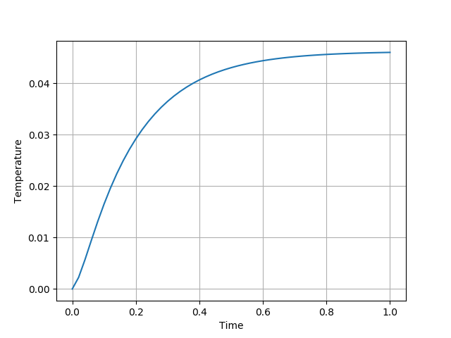
(d) The computational graph of the dynamical system can be efficiently constructed using while_loop. Implement the forward computation using while_loop. For debugging, you can plot the temperature on the left side, i.e., $u(0,t)$. You should have something similar to the following plot

(e) Now we are ready to perform inverse modeling. Read the starter code starter2.jlcarefully and complete the missing implementations. What is your estimate a and b?

Problem 2: Function Inverse Problem

Now let us consider the function inverse problem, where we do not know the form of $\kappa(x)$. To this end, we substitute $\kappa(x)$ using a neural network. We will use physics constrained learning (PCL) to train $\kappa(x)$ from the temperature data $u_0(t)$.

Since we do not know the form of $\kappa(x)$, it's reasonable we need more data to solve the inverse problem. Therefore, we assume that we place sensors at the first 25 locations in the discretized grid. The obervation data data_pcl.txt is a $(m+1)\times 25$ matrix, each column corresponds to the observation at one sensor.

In this problem, let us parametrize $\kappa(x)$ with a fully conneted neural network with 3 hidden layers, 20 neurons per layer, and $\tanh$ activation functions. In ADCME, such a neural network can be constructed using

y = fc(x, [20,20,20,1])

Here $\texttt{x}$ is a $n\times 1$ input, $\texttt{y}$ is a $n\times 1$ output, $[20,20,20,1]$ is the number of neurons per layer (last output layer only has 1 neuron), and $\texttt{fc}$ stands for "fully-connected".

(a) Assume that the neural network is written as $\kappa_\theta(x)$, where $\theta$ is the weights and biases. Write down the mathematical optimization problem for the inverse modeling.

(b) Complete the starter code for conducting physics constrained learning. The observation data is provided as data_pcl.txt. Run the program several times to ensure you do not terminate early at a bad local minimum. Plot your estimated $\kappa_\theta$ curve.

Hint: Your curve should look like the following

(c) Add 1% and 10% Gaussian noises to the dataset and redo (b), what do you find? Plot the estimated $\kappa_\theta$ curve.

Hint: You can add noises by

uc = @. uc * (1 + 0.01*randn(length(uc)))
uc = @. uc * (1 + 0.1*randn(length(uc)))

Here @. is for elementwise operations.

Problem 3: Parameter Inverse Problem in 2D

In this problem, we will digger deeper into how ADCME works with numerical solvers. We will use an important technique, custom operators, for incoporating C++ codes. This will be useful when you want to accelerate a performance critical part, or you want to reuse existing codes. To make the problem simple, the C++ kernel is prepared for you so what you need to do is to follow the instructions and call the custom operator.

We consider the 2D case and $T=1 $. We assume that $\Omega=[0,1]^2$. We impose zero boundary conditions on the entire boundary $\Gamma_D=\partial\Omega$. Additionally, we assume the initial condition is zero everywhere. Two sensors are located at (0.2,0.2) and $(0.8,0.8)$ and these sensors record time series of the temperature $u_1(t)$ and $u_2(t)$. The thermal diffusivity coefficient is a linear function of the space coordinates

where $a, b$ and $c$ are three coefficients we want to find out from the data $u_1(t)$ and $u_2(t)$.

(a) Write down the mathematical optimization problem for the inverse modeling.

We use the finite difference method to discretize the PDE. Consider $\Omega=[0,1]\times [0,1]$, we use a uniform grid and divide the domain into $m\times n$ squares, with length $\Delta x$. We also divide $[0,T]$ into $N_T$ intervals of equal length. The implicit scheme for the equation is

where $i=2,3,\ldots, m, j=2,3,\ldots, n, k=1,2,\ldots, N_T$.

Here $u_{ij}^k$ is an approximation to $u((i-1)h, (j-1)h, (k-1)\Delta t)$, and $f_{ij}^k = f((i-1)h, (j-1)h, (k-1)\Delta t)$.

We flatten $\{u_{ij}^k\}$ to a vector $U^k$, using $i$ as the leading dimension, i.e., the order is $u_{11}^k, u_{12}^k, \ldots$. We also flatten $f_{ij}^{k+1}$ and $\kappa_{ij}$ as well.

The following question reminds you of extending an AD framework using custom operators. In the starter code, we provide a function, heat_equation, a differentiable solver, which is already implemented for you using custom operators. Read the instruction on how to compile the custom operator, and answer the following two questions.

(b) Similar to Problem 1, implement forward computation using while_loop. Plot the curve of the temperature at $(0.5,0.5)$. For debugging, you should obtain something as follows

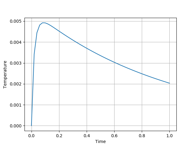
The parameters used in this problem: $m=50$, $n=50$, $T=1$, $N_T=50$, $f(\mathbf{x},t) = e^{-t}\exp(-50((x-0.5)^2+(y-0.5)^2))$, $a = 1.5$, $b=1.0$, $c=2.0$.

(c) The data file data.txt is a $(N_T+1)\times 2$ matrix, where the first and the second columns are $u_1(t)$ and $u_2(t)$ respectively. Using these data to do inverse modeling and report the values $a, b$ and $c$. We do not provide a starter code intentionally, but the forward computation codes in (b) and Problem 1 will be helpful.

Hint:

1. For checking your program, you can save your own data.txt from (b), try to estimate $a$, $b$, and $c$, and check if you can recover the true values.
2. If the optimization stop too early, you can multiply your loss function by a large number (e.g., $10^{10}$) and run your BFGS! optimizer again.