Numerical Scheme in ADCME: Finite Element Example

The purpose of this tutorial is to show how to work with the finite element method (FEM) in ADCME. The tutorial is divided into two part. In the first part, we implement a finite element code for 1D Poisson equation using ADCME without custom operators. In the first part, you will understand how while_loop can help avoid creating a computational graph for each element. This is important because for many applications the number of elements in FEM can be enormous. The goal of the second part is to introduce customop for FEM. For performance critical applications, you may want to code your own loop over elements. However, in this case, you are responsible to calculate the sensititity of your finite element sensitivity matrix.

Why do you need while loop?

In engineering, we usually need to do for loops, e.g., time stepping, finite element matrix assembling, etc. In pseudocode, we have

x = constant(0.0)
for i = 1:10000
  global x
	x = x + i 
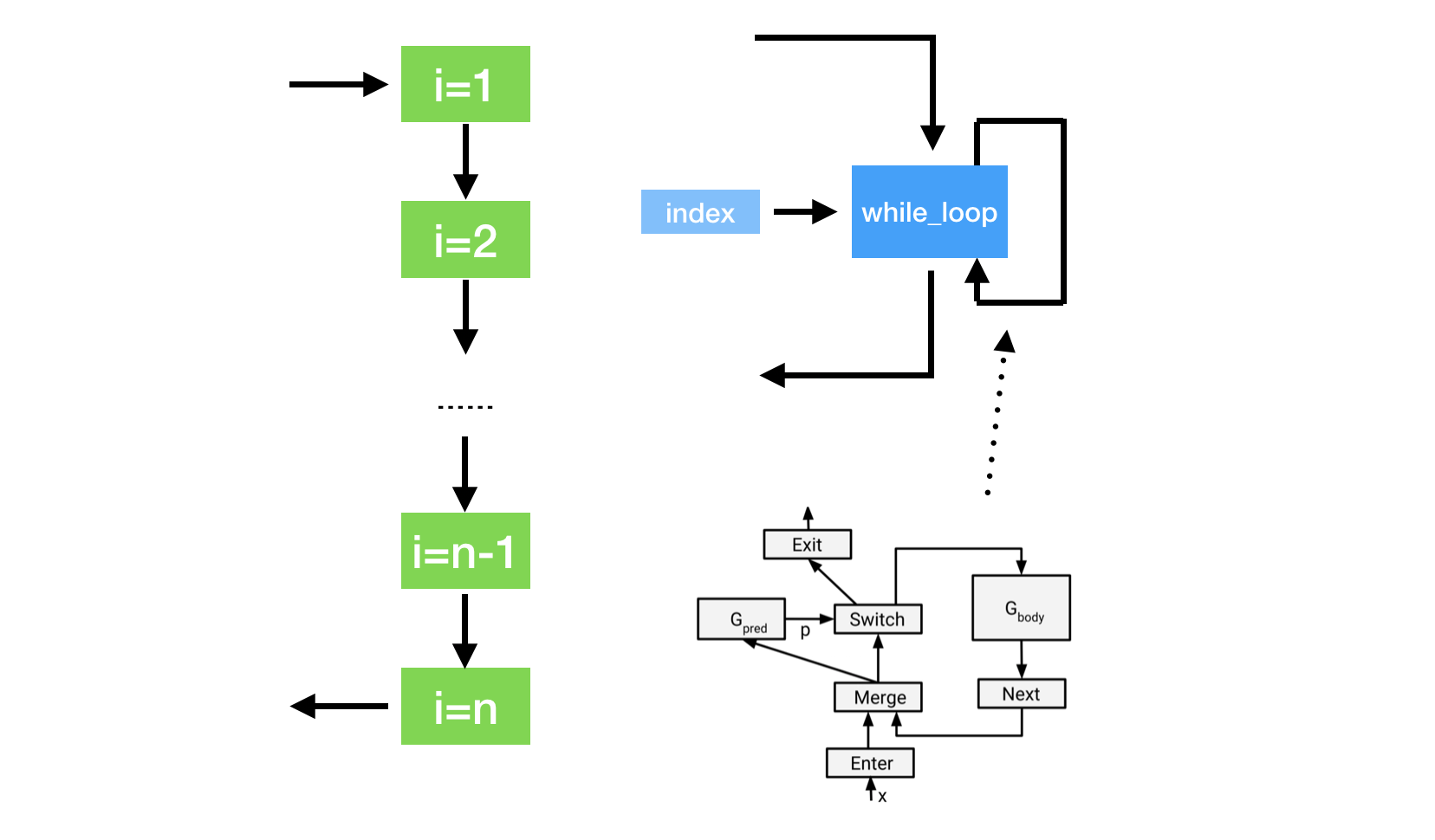
end

To do automatic differentiation in ADCME, direct implemnetation in the above way incurs creation of 10000 subgraphs, which requires large memories and long dependency parsing time.

Instead of relying on programming languages for the dynamic control flow, TensorFlow embeds control-flow as operations inside the dataflow graph. This is done via while_loop, which ADCME inherents from TensorFlow. while_loop allows for easier graph-based optimization, and reduces time and memory for the computational graph.

Using while_loop, the same function can be implemented as follows,

function func(i, ta)
  xold = read(ta, i)
  x = xold + cast(Float64, i)
  ta = write(ta, i+1, x)
  return i+1, ta
end
i = constant(1, dtype = Int32)
ta = TensorArray(10001)
ta = write(ta, 1, constant(0.0))
_, out = while_loop((i, x)->i<=10000, func, [i, ta])
result = stack(out)
sess = Session()
run(sess,result)

1D Example

As a simple example, we consider assemble the external load vector for linear finite elements in 1D. Assume that the load distribution is $f(x)=1-x^2$, $x\in[0,1]$. The goal is to compute a vector $\mathbf{v}$ with $v_i=\int_{0}^1 f(x)\phi_i(x)dx$, where $\phi_i(x)$ is the $i$-th linear element.

The pseudocode for this problem is shown in the following

F = zeros(ne+1) // ne is the total number of elements
for e = 1:ne
  add load contribution to F[e] and F[e+1]
end

However, if ne is very large, writing explicit loops is unwise since it will create ne subgraphs. while_loop can be very helpful in this case

using ADCME

ne = 100
h = 1/ne
f = x->1-x^2
function cond0(i, F_arr)
    i<=ne+1
end
function body(i, F_arr)
    fmid = f(cast(i-2, Float64)*h+h/2)
    F = vector([i-1;i], [fmid*h/2;fmid*h/2], ne+1)      # (1)
    F_arr = write(F_arr, i, F)
    i+1, F_arr
end

F_arr = TensorArray(ne+1)
F_arr = write(F_arr, 1, constant(zeros(ne+1))) # (2)
i = constant(2, dtype=Int32)
_, out = while_loop(cond0, body, [i,F_arr]; parallel_iterations=10)
F = sum(stack(out), dims=1)  # (3)
sess = Session(); init(sess)
F0 = run(sess, F)

Detailed explaination: (1) vector(idx, val, len) creates a length len vector with only the indices idx nonzero, populated with values val, i.e., v[idx] = val; (2) it is important to populate the first entry in a TensorArray, partially because of the need to inform F_arr of the data type; (3) stack extracts the output out as a tensor.

2D Example

In this section, we demonstrate how to assemble a finite element matrix based on while_loop for a 2D Poisson problem. We consider the following problem

\[\begin{aligned} \nabla \cdot ( D\nabla u(\mathbf{x}) ) &= f(\mathbf{x})& \mathbf{x}\in \Omega\\ u(\mathbf{x}) &= 0 & \mathbf{x}\in \partial \Omega \end{aligned}\]

Here $\Omega$ is the unit disk. We consider a simple case, where

\[\begin{aligned} D&=\mathbf{I}\\ f(\mathbf{x})&=-4 \end{aligned}\]

Then the exact solution will be

\[u(\mathbf{x}) = 1-x^2-y^2\]

The weak formulation is

\[\langle \nabla v(\mathbf{x}), D\nabla u(\mathbf{x}) \rangle = \langle f(\mathbf{x}),v(\mathbf{x}) \rangle\]

We split $\Omega$ into triangles $\mathcal{T}$ and use piecewise linear basis functions. Typically, we would iterate over all elements and compute the local stiffness matrix for each element. However, this could result in a large loop if we use a fine mesh. Instead, we can use while_loop to complete the task.

The implementation is split into two parts:

The first part is associated with data preprocessing such as precompute finite element data. The quantities in this part do not require gradients and therefore can leverage the full performance of Julia.
The second part is accociated with finite element. Particularly, the quantity of interest is $D$, which we may want to estimate from data in the future.

using ADCME, LinearAlgebra, PyCall
using DelimitedFiles
using PyPlot

# read data 
elem = readdlm("meshdata/elem.txt", Int64)
node = readdlm("meshdata/nodes.txt")
dof = readdlm("meshdata/dof.txt", Int64)[:]
elem_ = constant(elem)
ne = size(elem,1)
nv = size(node, 1)

# precompute 
localcoef = zeros(ne, 3, 3)
areas = zeros(ne)
for e = 1:ne 
    el = elem[e,:]
    x1, y1 = node[el[1],:]
    x2, y2 = node[el[2],:]
    x3, y3 = node[el[3],:]
    A = [x1 y1 1.0; x2 y2 1.0; x3 y3 1.0]
    localcoef[e,:,:] = inv(A)
    areas[e] = 0.5*abs(det(A))
end

# compute right hand side using midpoint rule 
rhs = zeros(nv)
for i = 1:ne
    el = elem[i,:]
    rhs[el] .+= 4*areas[i]/3
end

areas = constant(areas)
localcoef = constant(localcoef)
D = constant(diagm(0=>ones(2)))
function body(i, tai, taj, tav)
    el = elem_[i-1]
    a = areas[i-1]
    L = localcoef[i-1]
    LocalStiff = Array{PyObject}(undef, 3, 3)
    for i = 1:3
        for j = 1:3
            LocalStiff[i,j] = a*[L[1,i] L[2,i]]*D*[L[1,j];L[2,j]]|>squeeze
        end
    end
    ii = reshape([el el el], (-1,))
    jj = reshape([el;el;el], (-1,))
    tai = write(tai, i, ii)
    taj = write(taj, i, jj)
    # op = tf.print(el)
    # i = bind(i, op)
    tav = write(tav, i, vcat(LocalStiff[:]...))
    return i+1, tai, taj, tav 
end

i = constant(2, dtype=Int32)
tai = TensorArray(ne+1, dtype=Int64)
taj = TensorArray(ne+1, dtype=Int64)
tav = TensorArray(ne+1)
tai = write(tai, 1, constant(ones(Int64,9)))
taj = write(taj, 1, constant(ones(Int64,9)))
tav = write(tav, 1, constant(zeros(9)))
_, ii, jj, vv = while_loop((i, tas...)->i<=ne+1, body, [i, tai, taj, tav])
ii = reshape(stack(ii),(-1,)); jj = reshape(stack(jj),(-1,)); vv = reshape(stack(vv),(-1,))

A = SparseTensor(ii, jj, vv, nv, nv) # (1)

ndof = [x for x in setdiff(Set(1:nv), Set(dof))]
A = scatter_update(A, dof, ndof, spzero(length(dof), length(ndof)))  # (2)
A = scatter_update(A, ndof, dof, spzero(length(ndof), length(dof)))
A = scatter_update(A, dof, dof, spdiag(length(dof)))
rhs[dof] .= 0.0
sol = A\rhs  # (3)

sess = Session(); init(sess)
S = run(sess, sol)
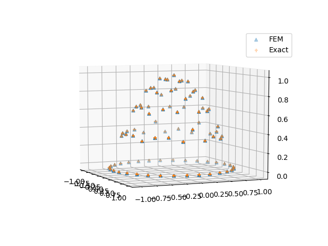
close("all")
scatter3D(node[:,1], node[:,2], S, marker="^", label = "FEM")
scatter3D(node[:,1], node[:,2], (@. 1-node[:,1]^2-node[:,2]^2), marker = "+", label = "Exact")
legend()

The implementation in the while_loop part is a standard routine in FEM. Other detailed explaination: (1) We use SparseTensor to create a sparse matrix out of the row indices, column indices and values. (2) scatter_update sets part of the sparse matrix to a given one. spzero and spdiag are convenient ways to specify zero and identity sparse matrices. (3) The backslash operator will invoke a sparse solver (the default is SparseLU).

Sensitivity

The gradients with respect to the parameters in the finite element coefficient matrix, also known as the sensitivity, can be computed using automatic differentiation. For example, to extract the sensitivity of the solution norm with respect to D, we have

gradients(sum(sol^2), D)

The output is a 2 by 2 sensitivity matrix.

Inversion

If we only know the discrete solution, and the form of $D=x\mathbf{I}$, $x>0$. This can be easily done by replacing D = constant(diagm(0=>ones(2))) with (the initial guess for $x=2$)

D = Variable(2.0) .* [1.0 0.0;0.0 1.0]

Then, we can estimate $x$ using L-BFGS-B

loss = sum((sol - (@. 1-node[:,1]^2-node[:,2]^2))^2)
sess = Session(); init(sess)
BFGS!(sess, loss)

The estimated result is

\[D = \begin{bmatrix}1.0028 & 0.0\\ 0.0 & 1.0028\end{bmatrix}\]

The Philosophy of Implementing Custom Operators

Usually the motivation for implementing custom operators is to enable gradient backpropagation for some performance critical operators. However, not all performance critical operators participate the automatic differentiation. Therefore, before we devote ourselves to implementating custom operators, we need to identify which operators need to be implemented as custom operators.

forwardbackward

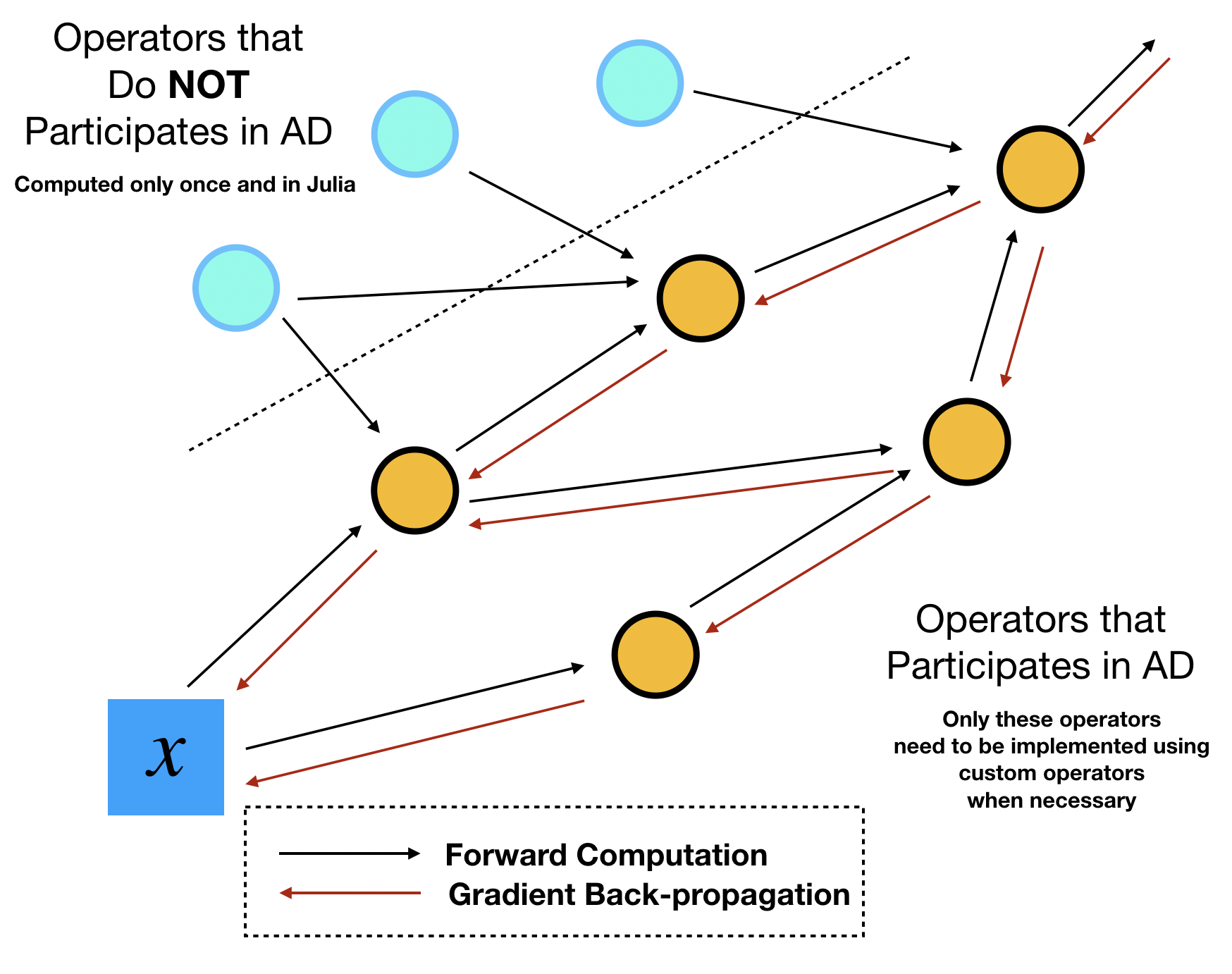
This identification task can be done by sketching out the computational graph of your program. Assume your optimization outer loops update $x$ repeatly, then we can trace all downstream the operators that depend on this parameter $x$. We call the dependent operators "tensor operations", because they are essentially TensorFlow operators that consume and output tensors. The dependent variables are called "tensors". The other side of tensors or tensor operations is "numerical arrays" and "numerical operations". The names seem a bit vague here but the essence is that numerical operations/arrays do no participate automatic differentiation during the optimization. They are essentially computed once.

In ADCME, we can precompute all numerical quantities of numerical arrays using Julia. No TensorFlow operators or custom operators are needed. This procedure combines the best of the two worlds: the simple syntax and high performance computing environment provided by Julia, and the efficient AD capability provided by TensorFlow. The high performance computing for precomputing cannot be provided by Python, the official language that TensorFlow or PyTorch supports. Readers migh suspect that such precomputing may not be significant in many tasks. Actually, the precomputing constitutes a large portion in scientific computing. For example, researchers assemble matrices, prepare geometries and construct preconditioners in a finite element program. These tasks are by no means trivial and cheap. The consideration for performance in scientific computing actually forms the major motivation behind adopting Julia for the major language for ADCME.

Summary

Finite element analysis is a powerful tool in numerical PDEs. However, it is more conceptually sophisticated than the finite difference method and requires more implementation efforts. The important lesson we learned from this tutorial is the necessity of while_loop, how to separate the computation into pure Julia and ADCME C++ kernels, and how complex numerical schemes can be implemented in ADCME.