API
Data Structures
AdFem.PoreData — Type.PoreData is a collection of physical parameters for coupled geomechanics and flow simulation
M: Biot modulusb: Biot coefficientρb: Bulk densityρf: Fluid densitykp: PermeabilityE: Young modulusν: Poisson ratioμ: Fluid viscosityPi: Initial pressureBf: formation volume, $B_f=\frac{\rho_{f,0}}{\rho_f}$g: Gravity acceleration
AdFem.Mesh — Type.Mesh holds data structures for an unstructured mesh.
nodes: a $n_v \times 2$ coordinates arrayedges: a $n_{\text{edge}} \times 2$ integer array for edgeselems: a $n_e \times 3$ connectivity matrix, 1-based.nnode,nedge,nelem: number of nodes, edges, and elementsndof: total number of degrees of freedomsconn: connectivity matrix,nelems × 3ornelems × 6, depending on whether a linear element or a quadratic element is used.lorder: order of quadrature rule for line integralselem_type: type of the element (P1, P2 or BDM1)
Internally, the mesh mmesh is represented by a collection of NNFEM_Element object with some other attributes
int nelem; // total number of elements
int nnode; // total number of nodes
int ngauss; // total number of Gauss points
int ndof; // total number of dofs
int order; // quadrature integration order
int degree; // Degree of Polynomials, 1 - P1 element, 2 - P2 element
int elem_ndof; // 3 for P1, 6 for P2
MatrixXd GaussPts; // coordinates of Gauss quadrature points
std::vector<NNFEM_Element*> elements; // array of elements
The NNFEM_Element has data
VectorXd h;   // basis functions, elem_ndof × ng
VectorXd hx;  // x-directional basis functions, elem_ndof × ng
VectorXd hy;  // y-directional basis functions, elem_ndof × ng
MatrixXd hs;  // shape functions for linear element, 3 × ng
VectorXd w;   // weight vectors, ng
double area;  // area of the triangle
MatrixXd coord; // coordinates array, 3 × 2
int nnode; // total number of nodes
int ngauss; // total number of Gauss points
int dof[6]; // global indices for both nodes and edges, note that edge indices are offset by `nv`
int node[3]; // global indices of local vertices
int edge[3]; // global indices of local edges
int ndof; // DOF, 3 for P1 element, 6 for P2 element
Matrix Assembling Functions
AdFem.compute_fem_stiffness_matrix — Function.compute_fem_stiffness_matrix(K::Array{Float64,2}, m::Int64, n::Int64, h::Float64)Computes the term
where the constitutive relation is given by
compute_fem_stiffness_matrix(hmat::PyObject,m::Int64, n::Int64, h::Float64)A differentiable kernel. hmat has one of the following sizes
- \[3\times 3\]
- \[4mn \times 3 \times 3\]
compute_fem_stiffness_matrix(kappa::PyObject, mesh::Mesh)
compute_fem_stiffness_matrix(kappa::Array{Float64, 3}, mesh::Mesh)
compute_fem_stiffness_matrix(kappa::Array{Float64, 2}, mesh::Mesh)
AdFem.compute_interaction_matrix — Function.compute_interaction_matrix(m::Int64, n::Int64, h::Float64)Computes the interaction term
Here $\varepsilon_v = \text{tr}\; \varepsilon = \text{div}\; \mathbf{u}$.
The output is a $mn \times 2(m+1)(n+1)$ matrix.
compute_interaction_matrix(mesh::Mesh)AdFem.compute_fvm_tpfa_matrix — Function.compute_fvm_tpfa_matrix(m::Int64, n::Int64, h::Float64)Computes the term with two-point flux approximation
No flow boundary condition is assumed.
compute_fvm_tpfa_matrix(K::Array{Float64}, m::Int64, n::Int64, h::Float64)Computes the term with two-point flux approximation with distinct permeability at each cell
Note that $K$ is a length $mn$ vector, representing values per cell.
compute_fvm_tpfa_matrix(K::Array{Float64}, bc::Array{Int64,2}, pval::Array{Float64,1}, m::Int64, n::Int64, h::Float64)Computes the term with two-point flux approximation with distinct permeability at each cell
Here $K$ is a length $mn$ vector, representing values per cell.
Additionally, Dirichlet boundary conditions are imposed on the boundary edges bc (a $N\times 2$ integer matrix), i.e., the $i$-th edge has value pval. The ghost node method is used for imposing the Dirichlet boundary condition. The other boundaries are no-blow boundaries, i.e., $\frac{\partial T}{\partial n} = 0$. The function outputs a length $mn$ vector and $mn\times mn$ matrix $M$.
Returns both the sparse matrix A and the right hand side rhs.
K can also be missing, in which case K is treated as a all-one vector.
compute_fvm_tpfa_matrix(K::PyObject, bc::Array{Int64,2}, pval::Union{Array{Float64},PyObject}, m::Int64, n::Int64, h::Float64)A differentiable kernel for compute_fvm_tpfa_matrix.
compute_fvm_tpfa_matrix(K::PyObject, m::Int64, n::Int64, h::Float64)A differentiable kernel for compute_fvm_tpfa_matrix.
AdFem.compute_fem_mass_matrix — Function.compute_fem_mass_matrix(m::Int64, n::Int64, h::Float64)Computes the finite element mass matrix
The matrix size is $2(m+1)(n+1) \times 2(m+1)(n+1)$.
compute_fem_mass_matrix(ρ::PyObject,m::Int64, n::Int64, h::Float64)A differentiable kernel. $\rho$ is a vector of length $4mn$ or $8mn$
AdFem.compute_fvm_mass_matrix — Function.compute_fvm_mass_matrix(m::Int64, n::Int64, h::Float64)Returns the FVM mass matrix
AdFem.compute_fem_mass_matrix1 — Function.compute_fem_mass_matrix1(ρ::Array{Float64,1}, m::Int64, n::Int64, h::Float64)Computes the mass matrix for a scalar value $u$
The output is a $(m+1)(n+1)\times (m+1)(n+1)$ sparse matrix.
compute_fem_mass_matrix1(m::Int64, n::Int64, h::Float64)Computes the mass matrix for a scalar value $u$
The output is a $(m+1)(n+1)\times (m+1)(n+1)$ sparse matrix.
compute_fem_mass_matrix1(ρ::PyObject,m::Int64, n::Int64, h::Float64)A differentiable kernel.
compute_fem_mass_matrix1(rho::Union{PyObject, Array{Float64, 1}}, mesh::Mesh)AdFem.compute_fem_stiffness_matrix1 — Function.compute_fem_stiffness_matrix1(K::Array{Float64,2}, m::Int64, n::Int64, h::Float64)Computes the term
Returns a $(m+1)\times (n+1)$ matrix
compute_fem_stiffness_matrix1(hmat::PyObject, m::Int64, n::Int64, h::Float64)A differentiable kernel for computing the stiffness matrix. Two possible shapes for hmat are supported:
- \[4mn \times 2\times 2\]
- \[2 \times 2\]
AdFem.compute_fvm_advection_matrix — Function.compute_fvm_advection_matrix(v::Union{PyObject, Array{Float64, 2}},
bc::Array{Int64, 2},bcval::Union{PyObject, Array{Float64}},m::Int64,n::Int64,h::Float64)Computes the advection matrix for use in the implicit scheme
Here v is a $2mn$ vector, where the first $mn$ entries corresponds to the first dimension of $\mathbf{v}$ and the remaining $mn$ entries corresponds to the second dimension.
It returns a matrix $mn\times mn$ matrix $K$ and an auxilliary term $\mathbf{f}$ due to boundary conditions.
AdFem.compute_fem_laplace_matrix1 — Function.compute_fem_laplace_matrix1(K::Array{Float64, 1}, m::Int64, n::Int64, h::Float64)Computes the coefficient matrix for
Here $K\in \mathbf{R}^{2\times 2}$, $u$ is a scalar variable, and K is a $4mn \times 2 \times 2$ matrix.
Returns a $(m+1)(n+1)\times (m+1)(n+1)$ sparse matrix.
compute_fem_laplace_matrix1(K::Array{Float64, 2}, m::Int64, n::Int64, h::Float64)K is duplicated on each Gauss point.
compute_fem_laplace_matrix1(K::Array{Float64, 1}, m::Int64, n::Int64, h::Float64)Computes the coefficient matrix for
Here K is a vector with length $4mn$ (defined on Gauss points).
Returns a $(m+1)(n+1)\times (m+1)(n+1)$ sparse matrix.
compute_fem_laplace_matrix1(m::Int64, n::Int64, h::Float64)Computes the coefficient matrix for
Returns a $(m+1)(n+1)\times (m+1)(n+1)$ sparse matrix.
compute_fem_laplace_matrix1(K::PyObject, m::Int64, n::Int64, h::Float64)A differentiable kernel. Only $K\in \mathbb{R}^{4mn}$ is supported.
compute_fem_laplace_matrix1(kappa::PyObject, mesh::Mesh)compute_fem_laplace_matrix1(kappa::Array{Float64,1}, mesh::Mesh)AdFem.compute_fem_laplace_matrix — Function.compute_fem_laplace_matrix(m::Int64, n::Int64, h::Float64)Computes the coefficient matrix for
Here
and
Returns a $2(m+1)(n+1)\times 2(m+1)(n+1)$ sparse matrix.
compute_fem_laplace_matrix(K::Array{Float64, 1}, m::Int64, n::Int64, h::Float64)Computes the coefficient matrix for
Here $K$ is a scalar defined on Gauss points. K is a vector of length $4mn$
compute_fem_laplace_matrix(kappa::Union{PyObject, Array{Float64, 1}}, mesh::Mesh)AdFem.compute_fem_advection_matrix1 — Function.compute_fem_advection_matrix1(u0::PyObject,v0::PyObject,m::Int64,n::Int64,h::Float64)Computes the advection term for a scalar function $u$ defined on an FEM grid. The weak form is
Here $u_0$ and $v_0$ are both vectors of length $4mn$.
Returns a sparse matrix of size $(m+1)(n+1)\times (m+1)(n+1)$
compute_fem_advection_matrix1(u::Union{Array{Float64,1}, PyObject},v::Union{Array{Float64,1}, PyObject}, mesh::Mesh)
compute_fem_advection_matrix1(u::Array{Float64,1}, v::Array{Float64,1}, mesh::Mesh)
AdFem.compute_fem_bdm_mass_matrix — Function.compute_fem_bdm_mass_matrix(alpha::Union{Array{Float64,1}, PyObject},beta::Union{Array{Float64,1}, PyObject}, mmesh::Mesh)Computes
Here
Here $\sigma$ and $\tau$ are both fourth-order tensors. The output is a 4mmesh.nedge × 4mmesh.nedge matrix.
compute_fem_bdm_mass_matrix(mmesh::Mesh)Same as compute_fem_bdm_mass_matrix
compute_fem_bdm_mass_matrix(alpha::Array{Float64,1},beta::Array{Float64,1}, mmesh::Mesh)AdFem.compute_fem_bdm_mass_matrix1 — Function.compute_fem_bdm_mass_matrix1(alpha::Array{Float64,1}, mmesh::Mesh)Computes
Here $\alpha$ is a scalar, and $\sigma$ and $\delta \tau$ are second order tensors.
The returned value is a 2mmesh.nedge × 2mmesh.nedge matrix.
compute_fem_bdm_mass_matrix1(mmesh::Mesh)Same as compute_fem_bdm_mass_matrix1, except that $\alpha\equiv 1$
AdFem.compute_fem_bdm_div_matrix — Function.compute_fem_bdm_div_matrix(mmesh::Mesh)Computes the coefficient matrix for
Here $\tau \in \mathbb{R}^{2\times 2}$ is a fourth-order tensor (not necessarily symmetric). mmesh uses the BDM1 finite element. The output is a 2mmesh.nelem × 4mmesh.nedge matrix.
AdFem.compute_fem_bdm_div_matrix1 — Function.compute_fem_bdm_div_matrix1(mmesh::Mesh)Computes the coefficient matrix for
Here $\tau \in \mathbb{R}^{2}$ is a second-order tensor (not necessarily symmetric). mmesh uses the BDM1 finite element. The output is a mmesh.nelem × 2mmesh.nedge matrix.
AdFem.compute_fem_bdm_skew_matrix — Function.compute_fem_bdm_skew_matrix(mmesh::Mesh)Computes $\int_\Omega \sigma : v dx$ where
Here $\sigma$ is a fourth-order tensor.
The returned value is a mmesh.nelem × 4mmesh.nedge matrix.
Vector Assembling Functions
AdFem.compute_fem_source_term — Function.compute_fem_source_term(f1::Array{Float64}, f2::Array{Float64},
m::Int64, n::Int64, h::Float64)Computes the term
Returns a $2(m+1)(n+1)$ vector.
compute_fem_source_term(f1::PyObject, f2::PyObject,
m::Int64, n::Int64, h::Float64)
A differentiable kernel.
compute_fem_source_term(f1::Union{PyObject,Array{Float64,2}}, f2::Union{PyObject,Array{Float64,2}}, mesh::Mesh)AdFem.compute_fvm_source_term — Function.compute_fvm_source_term(f::Array{Float64}, m::Int64, n::Int64, h::Float64)Computes the source term
Here $f$ has length $4mn$ or $mn$. In the first case, an average value of four quadrature nodal values of $f$ is used per cell.
compute_fvm_source_term(f::PyObject, m::Int64, n::Int64, h::Float64)A differentiable kernel.
compute_fvm_source_term(f::Array{Float64, 1}, mmesh::Mesh)AdFem.compute_fvm_mechanics_term — Function.compute_fvm_mechanics_term(u::Array{Float64}, m::Int64, n::Int64, h::Float64)Computes the mechanic interaction term
Here
Numerically, we have
compute_fvm_mechanics_term(u::PyObject, m::Int64, n::Int64, h::Float64)AdFem.compute_fem_normal_traction_term — Function.compute_fem_normal_traction_term(t::Array{Float64,1}, bdedge::Array{Int64},
m::Int64, n::Int64, h::Float64)
compute_fem_normal_traction_term(t::Float64, bdedge::Array{Int64},
m::Int64, n::Int64, h::Float64)Computes the normal traction term
Here $t(\mathbf{n})\parallel\mathbf{n}$ points outward to the domain and the magnitude is given by t. bdedge is a $N\times2$ matrix and each row denotes the indices of two endpoints of the boundary edge.
See compute_fem_traction_term for graphical illustration.
AdFem.compute_fem_traction_term — Function.compute_fem_traction_term(t::Array{Float64, 2},
bdedge::Array{Int64,2}, m::Int64, n::Int64, h::Float64)Computes the traction term
The number of rows of t is equal to the number of edges in bdedge. The first component of t describes the $x$ direction traction, while the second component of t describes the $y$ direction traction.
Also see compute_fem_normal_traction_term.

compute_fem_traction_term(t::Array{Float64, 2},
bdedge::Array{Int64,2}, mesh::Mesh)
compute_fem_traction_term(t1::Array{Float64, 1}, t2::Array{Float64, 1},
bdedge::Array{Int64,2}, mesh::Mesh)AdFem.compute_von_mises_stress_term — Function.compute_von_mises_stress_term(K::Array{Float64}, u::Array{Float64}, m::Int64, n::Int64, h::Float64)Compute the von Mises stress on the Gauss quadrature nodes.
compute_von_mises_stress_term(Se::Array{Float64,2}, m::Int64, n::Int64, h::Float64)Se is a $4mn\times3$ array that stores the stress data at each Gauss point.
compute_von_mises_stress_term(K::Array{Float64, 3}, u::Array{Float64, 1}, mesh::Mesh)
compute_von_mises_stress_term(K::Array{Float64, 2}, u::Array{Float64, 1}, mesh::Mesh)
AdFem.compute_fem_source_term1 — Function.compute_fem_source_term1(f::Array{Float64},
m::Int64, n::Int64, h::Float64)Computes the term
Returns a $(m+1)\times (n+1)$ vector. f is a length $4mn$ vector, given by its values on Gauss points.
compute_fem_source_term1(f::PyObject,
m::Int64, n::Int64, h::Float64)
A differentiable kernel.
compute_fem_source_term1(f::PyObject, mesh::Mesh)compute_fem_source_term1(f::Array{Float64,1}, mesh::Mesh)AdFem.compute_fem_flux_term1 — Function.compute_fem_flux_term1(t::Array{Float64},
bdedge::Array{Int64,2}, m::Int64, n::Int64, h::Float64)Computes the traction term
AdFem.compute_strain_energy_term — Function.compute_strain_energy_term(S::Array{Float64, 2}, m::Int64, n::Int64, h::Float64)Computes the strain energy
where $\sigma$ is provided by S, a $4mn \times 3$ matrix. The values $\sigma_{11}, \sigma_{22}, \sigma_{12}$ are defined on 4 Gauss points per element.
compute_strain_energy_term(S::PyObject,m::Int64, n::Int64, h::Float64)A differentiable kernel.
compute_strain_energy_term(Sigma::Array{Float64, 2}, mmesh::Mesh)Computes the strain energy term
Here $\sigma$ is a fourth-order tensor. Sigma is a ngauss × 3 matrix, each row represents $[\sigma_{11}, \sigma_{22}, \sigma_{12}]$ at each Gauss point.
The output is a length 2mmesh.ndof vector.
compute_strain_energy_term(Sigma::PyObject, mmesh::Mesh)AdFem.compute_strain_energy_term1 — Function.compute_strain_energy_term1(S::PyObject, m::Int64, n::Int64, h::Float64)Computes the strain energy
where $\sigma$ is provided by S, a $4mn \times 2$ matrix. The values $\sigma_{31}, \sigma_{32}$ are defined on 4 Gauss points per element.
compute_strain_energy_term1(sigma::PyObject, m::Int64, n::Int64, h::Float64)A differentiable operator.
compute_fem_viscoelasticity_strain_energy_term(ε0, σ0, ε, A, B, m, n, h)Given the constitutive relation
this function computes
and returns $f$
AdFem.compute_fvm_advection_term — Function.compute_fvm_advection_term(v::Union{PyObject, Array{Float64, 2}},
u::Union{PyObject, Array{Float64,1}},m::Int64,n::Int64,h::Float64)Computes the advection term using upwind schemes
Here $\mathbf{v}$ is a $mn\times 2$ matrix and $u$ is a length $mn$ vector. Zero boundary conditions are assumed. $u$ is a vector of length $m\times n$.
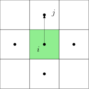
AdFem.compute_interaction_term — Function.compute_interaction_term(p::Array{Float64, 1}, m::Int64, n::Int64, h::Float64)Computes the FVM-FEM interaction term
The input is a vector of length $mn$. The output is a $2(m+1)(n+1)$ vector.
compute_interaction_term(p::PyObject, m::Int64, n::Int64, h::Float64)A differentiable kernel.
compute_interaction_term(p::Union{PyObject,Array{Float64, 1}}, mesh::Mesh)AdFem.compute_fem_laplace_term1 — Function.compute_fem_laplace_term1(u::PyObject,κ::PyObject,m::Int64,n::Int64,h::Float64)
compute_fem_laplace_term1(u::PyObject,m::Int64,n::Int64,h::Float64)
compute_fem_laplace_term1(u::Array{Float64},κ::PyObject, m::Int64,n::Int64,h::Float64)
compute_fem_laplace_term1(u::PyObject,κ::Array{Float64}, m::Int64,n::Int64,h::Float64)Computes the Laplace term for a scalar function $u$
Here κ is a vector of length $4mn$, and u is a vector of length $(m+1)(n+1)$.
When κ is not provided, the following term is calculated:
compute_fem_laplace_term1(u::Array{Float64, 1},nu::Array{Float64, 1}, mesh::Mesh)compute_fem_laplace_term1(u::Union{PyObject, Array{Float64, 1}},
nu::Union{PyObject, Array{Float64, 1}},
mesh::Mesh)AdFem.compute_fem_traction_term1 — Function.compute_fem_traction_term1(t::Array{Float64, 2},
bdedge::Array{Int64,2}, m::Int64, n::Int64, h::Float64)Computes the traction term
The number of rows of t is equal to the number of edges in bdedge. The output is a length $(m+1)*(n+1)$ vector.
Also see compute_fem_traction_term.
compute_fem_traction_term1(t::Array{Float64, 1},
bdedge::Array{Int64,2}, mesh::Mesh)
Computes the boundary integral
Returns a vector of size dof.
Evaluation Functions
AdFem.eval_f_on_gauss_pts — Function.eval_f_on_gauss_pts(f::Function, m::Int64, n::Int64, h::Float64; tensor_input::Bool = false)Evaluates f at Gaussian points and return the result as $4mn$ vector out (4 Gauss points per element)
If tensor_input = true, the function f is assumed to map a tensor to a tensor output.

eval_f_on_gauss_pts(f::Function, mesh::Mesh; tensor_input::Bool = false)AdFem.eval_f_on_dof_pts — Function.eval_f_on_dof_pts(f::Function, mesh::Mesh)Evaluates f on the DOF points.
- For P1 element, the DOF points are FEM points and therefore
eval_f_on_dof_ptsis equivalent toeval_on_on_fem_pts. - For P2 element, the DOF points are FEM points plus the middle point for each edge.
Returns a vector of length mesh.ndof.
AdFem.eval_f_on_boundary_node — Function.eval_f_on_boundary_node(f::Function, bdnode::Array{Int64}, m::Int64, n::Int64, h::Float64)Returns a vector of the same length as bdnode whose entries corresponding to bdnode nodes are filled with values computed from f.
f has the following signature
f(x::Float64, y::Float64)::Float64eval_f_on_boundary_node(f::Function, bdnode::Array{Int64}, mesh::Mesh)AdFem.eval_f_on_boundary_edge — Function.eval_f_on_boundary_edge(f::Function, bdedge::Array{Int64,2}, m::Int64, n::Int64, h::Float64)Returns a vector of the same length as bdedge whose entries corresponding to bdedge nodes are filled with values computed from f.
f has the following signature
f(x::Float64, y::Float64)::Float64eval_f_on_boundary_edge(f::Function, bdedge::Array{Int64, 2}, mesh::Mesh; tensor_input::Bool = false)Evaluates f on the boundary Gauss points. Here f has the signature
f(Float64, Float64)::Float64
or
f(PyObject, PyObject)::PyObject
AdFem.eval_strain_on_gauss_pts — Function.eval_strain_on_gauss_pts(u::Array{Float64}, m::Int64, n::Int64, h::Float64)Computes the strain on Gauss points. Returns a $4mn\times3$ matrix, where each row denotes $(\varepsilon_{11}, \varepsilon_{22}, 2\varepsilon_{12})$ at the corresponding Gauss point.
eval_strain_on_gauss_pts(u::PyObject, m::Int64, n::Int64, h::Float64)A differentiable kernel.
eval_strain_on_gauss_pts(u::Array{Float64}, mmesh::Mesh)Evaluates the strain on Gauss points. u is a vector of size 2mmesh.ndof.
The output is a ngauss × 3 vector.
eval_strain_on_gauss_pts(u::PyObject, mmesh::Mesh)AdFem.eval_strain_on_gauss_pts1 — Function.eval_strain_on_gauss_pts1(u::PyObject, m::Int64, n::Int64, h::Float64)A differentiable kernel.
AdFem.eval_f_on_fvm_pts — Function.eval_f_on_fvm_pts(f::Function, m::Int64, n::Int64, h::Float64; tensor_input::Bool = false)Returns $f(x_i, y_i)$ where $(x_i,y_i)$ are FVM nodes.
If tensor_input = true, the function f is assumed to map a tensor to a tensor output.
eval_f_on_fvm_pts(f::Function, mesh::Mesh; tensor_input::Bool = false)AdFem.eval_f_on_fem_pts — Function.eval_f_on_fem_pts(f::Function, m::Int64, n::Int64, h::Float64; tensor_input::Bool = false)Returns $f(x_i, y_i)$ where $(x_i,y_i)$ are FEM nodes.
If tensor_input = true, the function f is assumed to map a tensor to a tensor output.
eval_f_on_fem_pts(f::Function, mesh::Mesh; tensor_input::Bool = false)AdFem.eval_grad_on_gauss_pts1 — Function.eval_grad_on_gauss_pts1(u::Array{Float64,1}, m::Int64, n::Int64, h::Float64)Evaluates $\nabla u$ on each Gauss point. Here $u$ is a scalar function.
The input u is a vector of length $(m+1)*(n+1)$. The output is a matrix of size $4mn\times 2$.
eval_grad_on_gauss_pts1(u::PyObject, m::Int64, n::Int64, h::Float64)A differentiable kernel.
eval_grad_on_gauss_pts1(u::Union{Array{Float64,1}, PyObject}, mesh::Mesh)AdFem.eval_grad_on_gauss_pts — Function.eval_grad_on_gauss_pts(u::Array{Float64,1}, m::Int64, n::Int64, h::Float64)Evaluates $\nabla u$ on each Gauss point. Here $\mathbf{u} = (u, v)$.
The input u is a vector of length $2(m+1)*(n+1)$. The output is a matrix of size $4mn\times 2 \times 2$.
eval_grad_on_gauss_pts(u::PyObject, m::Int64, n::Int64, h::Float64)A differentiable kernel.
Boundary Conditions
AdFem.fem_impose_Dirichlet_boundary_condition — Function.fem_impose_Dirichlet_boundary_condition(A::SparseMatrixCSC{Float64,Int64},
bd::Array{Int64}, m::Int64, n::Int64, h::Float64)Imposes the Dirichlet boundary conditions on the matrix A.
Returns 2 matrix,
fem_impose_Dirichlet_boundary_condition(L::SparseTensor, bdnode::Array{Int64}, m::Int64, n::Int64, h::Float64)A differentiable kernel for imposing the Dirichlet boundary of a vector-valued function.
AdFem.fem_impose_Dirichlet_boundary_condition1 — Function.fem_impose_Dirichlet_boundary_condition1(A::SparseMatrixCSC{Float64,Int64},
bd::Array{Int64}, m::Int64, n::Int64, h::Float64)Imposes the Dirichlet boundary conditions on the matrix A Returns 2 matrix,
bd must NOT have duplicates.
fem_impose_Dirichlet_boundary_condition1(L::SparseTensor, bdnode::Array{Int64}, m::Int64, n::Int64, h::Float64)A differentiable kernel for imposing the Dirichlet boundary of a scalar-valued function.
fem_impose_Dirichlet_boundary_condition1(L::SparseTensor, bdnode::Array{Int64}, mesh::Mesh)A differentiable kernel for imposing the Dirichlet boundary of a scalar-valued function.
AdFem.impose_Dirichlet_boundary_conditions — Function.impose_Dirichlet_boundary_conditions(A::Union{SparseArrays, Array{Float64, 2}}, rhs::Array{Float64,1}, bdnode::Array{Int64, 1},
bdval::Array{Float64,1})
impose_Dirichlet_boundary_conditions(A::SparseTensor, rhs::Union{Array{Float64,1}, PyObject}, bdnode::Array{Int64, 1},
bdval::Union{Array{Float64,1}, PyObject})Algebraically impose the Dirichlet boundary conditions. We want the solutions at indices bdnode to be bdval. Given the matrix and the right hand side
The function returns
AdFem.impose_bdm_traction_boundary_condition1 — Function.impose_bdm_traction_boundary_condition1(gN::Array{Float64, 1}, bdedge::Array{Int64, 2}, mesh::Mesh)Imposes the BDM traction boundary condition
Here $\sigma$ is a second-order tensor. gN is defined on the Gauss points, e.g.
gN = eval_f_on_boundary_edge(func, bdedge, mesh)AdFem.impose_bdm_traction_boundary_condition — Function.impose_bdm_traction_boundary_condition(g1:Array{Float64, 1}, g2:Array{Float64, 1},
bdedge::Array{Int64, 2}, mesh::Mesh)Imposes the BDM traction boundary condition
Here $\sigma$ is a fourth-order tensor. $\mathbf{g}_N = \begin{bmatrix}g_{N1}\\ g_{N2}\end{bmatrix}$ See impose_bdm_traction_boundary_condition1.
Returns a dof vector and a val vector.
Visualization
In visualize_scalar_on_XXX_points, the first argument is the data matrix. When the data matrix is 1D, one snapshot is plotted. When the data matrix is 2D, it is understood as multiple snapshots at different time steps (each row is a snapshot). When the data matrix is 3D, it is understood as time step × height × width.
AdFem.visualize_mesh — Function.visualize_mesh(mesh::Mesh)Visualizes the unstructured meshes.
AdFem.visualize_pressure — Function.visualize_pressure(U::Array{Float64, 2}, m::Int64, n::Int64, h::Float64)Visualizes pressure. U is the solution vector.
AdFem.visualize_displacement — Function.visualize_displacement(u::Array{Float64, 2}, m::Int64, n::Int64, h::Float64)Generates scattered plot animation for displacement $u\in \mathbb{R}^{(NT+1)\times 2(m+1)(n+1)}$.
visualize_displacement(u::Array{Float64, 1}, mmesh::Mesh)visualize_displacement(u::Array{Float64, 2}, mmesh::Mesh)Generates scattered plot animation for displacement $u\in \mathbb{R}^{(NT+1)\times 2N_{\text{dof}}}$.
AdFem.visualize_stress — Function.visualize_stress(K::Array{Float64, 2}, U::Array{Float64, 2}, m::Int64, n::Int64, h::Float64; name::String="")Visualizes displacement. U is the solution vector, K is the elasticity matrix ($3\times 3$).
visualize_stress(Se::Array{Float64, 2}, m::Int64, n::Int64, h::Float64; name::String="")Visualizes the Von Mises stress. Se is the Von Mises at the cell center.
AdFem.visualize_von_mises_stress — Function.visualize_von_mises_stress(Se::Array{Float64, 2}, m::Int64, n::Int64, h::Float64; name::String="")Visualizes the Von Mises stress.
visualize_von_mises_stress(K::Array{Float64}, u::Array{Float64, 1}, mmesh::Mesh, args...; kwargs...)AdFem.visualize_scalar_on_gauss_points — Function.visualize_scalar_on_gauss_points(u::Array{Float64,1}, m::Int64, n::Int64, h::Float64, args...;kwargs...)Visualizes the scalar u using pcolormesh. Here u is a length $4mn$ vector and the values are defined on the Gauss points
visualize_scalar_on_gauss_points(u::Array{Float64,1}, mesh::Mesh, args...;kwargs...)Visualizes scalar values on Gauss points. For unstructured meshes, the values on each element are averaged to produce a uniform value for each element.
AdFem.visualize_scalar_on_fem_points — Function.visualize_scalar_on_fem_points(u::Array{Float64,1}, m::Int64, n::Int64, h::Float64, args...;kwargs...)Visualizes the scalar u using pcolormesh. Here u is a length $(m+1)(n+1)$ vector and the values are defined on the FEM points
visualize_scalar_on_fem_points(u::Array{Float64,2}, m::Int64, n::Int64, h::Float64, args...;kwargs...)Visualizes the scalar u using pcolormesh. Here u is a matrix of size $NT \times (m+1)(n+1)$ ($NT$ is the number of time steps) and the values are defined on the FEM points.
visualize_scalar_on_fem_points(u::Array{Float64,1}, mesh::Mesh, args...;
    with_mesh::Bool = false, kwargs...)
Visualizes the nodal values u on the unstructured mesh mesh.
with_mesh: if true, the unstructured mesh is also plotted.
AdFem.visualize_scalar_on_fvm_points — Function.visualize_scalar_on_fvm_points(φ::Array{Float64, 3}, m::Int64, n::Int64, h::Float64;
vmin::Union{Real, Missing} = missing, vmax::Union{Real, Missing} = missing)Generates scattered potential animation for the potential $\phi\in \mathbb{R}^{(NT+1)\times n \times m}$.
visualize_scalar_on_fvm_points(u::Array{Float64,1}, mesh::Mesh, args...;kwargs...)AdFem.visualize_vector_on_fem_points — Function.visualize_vector_on_fem_points(u1::Array{Float64,1}, u2::Array{Float64,1}, mesh::Mesh, args...;kwargs...)Modeling Tools
AdFem.layer_model — Function.layer_model(u::Array{Float64, 1}, m::Int64, n::Int64, h::Float64)Convert the vertical profile of a quantity to a layer model. The input u is a length $n$ vector, the output is a length $4mn$ vector, representing the $4mn$ Gauss points.
layer_model(u::PyObject, m::Int64, n::Int64, h::Float64)A differential kernel for layer_model.
AdFem.compute_vel — Function.compute_vel(a::Union{PyObject, Array{Float64, 1}},
v0::Union{PyObject, Float64},psi::Union{PyObject, Array{Float64, 1}},
sigma::Union{PyObject, Array{Float64, 1}},
tau::Union{PyObject, Array{Float64, 1}},eta::Union{PyObject, Float64})Computes $x = u_3(x_1, x_2)$ from rate and state friction. The governing equation is
AdFem.compute_plane_strain_matrix — Function.compute_plane_strain_matrix(E::Float64, ν::Float64)Computes the stiffness matrix for 2D plane strain. The matrix is given by
compute_plane_strain_matrix(E::Union{PyObject, Array{Float64, 1}}, nu::Union{PyObject, Array{Float64, 1}})AdFem.compute_plane_stress_matrix — Function.compute_plane_stress_matrix(E::Float64, ν::Float64)Computes the stiffness matrix for 2D plane stress. The matrix is given by
compute_plane_stress_matrix(E::Union{PyObject, Array{Float64, 1}}, nu::Union{PyObject, Array{Float64, 1}})compute_space_varying_tangent_elasticity_matrix(mu::Union{PyObject, Array{Float64,1}},m::Int64,n::Int64,h::Float64,type::Int64=1)Computes the space varying tangent elasticity matrix given $\mu$. It returns a matrix of size $4mn\times 2\times 2$
- If
type==1, the $i$-th matrix will be
- If
type==2, the $i$-th matrix will be
- If
type==3, the $i$-th matrix will be
AdFem.mantle_viscosity — Function.mantle_viscosity(u::Union{Array{Float64}, PyObject},
T::Union{Array{Float64}, PyObject}, m::Int64, n::Int64, h::Float64;
σ_yield::Union{Float64, PyObject} = 300e6,
ω::Union{Float64, PyObject},
η_min::Union{Float64, PyObject} = 1e18,
η_max::Union{Float64, PyObject} = 1e23,
E::Union{Float64, PyObject} = 9.0,
C::Union{Float64, PyObject} = 1000., N::Union{Float64, PyObject} = 2.)with
Here $\epsilon_{II}$ is the second invariant of the strain rate tensor, $C > 0$ is a viscosity pre-factor, $E > 0$ is the non-dimensional activation energy, $n > 0$ is the nonlinear exponent, $η_\min$, $η_\max$ act as minimum and maximum bounds for the effective viscosity, and $σ_{\text{yield}} > 0$ is the yield stress. $w\in (0, 1]$ is the weakening factor, which is used to incorporate phenomenological aspects that cannot be represented in a purely viscous flow model, such as processes which govern mega-thrust faults along the subduction interface, or partial melting near a mid-ocean ridge.
The viscosity of the mantle is governed by the high-temperature creep of silicates, for which laboratory experiments show that the creep strength is temperature-, pressure-, compositional- and stress-dependent.
The output is a length $4mn$ vector.
See Towards adjoint-based inversion of time-dependent mantle convection with nonlinear viscosity for details.
AdFem.antiplane_viscosity — Function.antiplane_viscosity(ε::Union{PyObject, Array{Float64}}, σ::Union{PyObject, Array{Float64}},
μ::Union{PyObject, Float64}, η::Union{PyObject, Float64}, Δt::Float64)Calculates the stress at time $t_{n+1}$ given the strain at $t_{n+1}$ and stress at $t_{n}$. The governing equation is
The discretization form is
AdFem.update_stress_viscosity — Function.update_stress_viscosity(ε2::Array{Float64,2}, ε1::Array{Float64,2}, σ1::Array{Float64,2},
invη::Array{Float64,1}, μ::Array{Float64,1}, λ::Array{Float64,1}, Δt::Float64)Updates the stress for the Maxwell model
See here for details.
update_stress_viscosity(ε2::Union{PyObject,Array{Float64,2}}, ε1::Union{PyObject,Array{Float64,2}}, σ1::Union{PyObject,Array{Float64,2}},
invη::Union{PyObject,Array{Float64,1}}, μ::Union{PyObject,Array{Float64,1}}, λ::Union{PyObject,Array{Float64,1}}, Δt::Union{PyObject,Float64})
Mesh
AdFem.get_edge_dof — Function.get_edge_dof(edges::Array{Int64, 2}, mesh::Mesh)
get_edge_dof(edges::Array{Int64, 1}, mesh::Mesh)Returns the DOFs for edges, which is a K × 2 array containing vertex indices. The DOFs are not offset by nnode, i.e., the smallest edge DOF could be 1.
When the input is a length 2 vector, it returns a single index for the corresponding edge DOF.
AdFem.get_boundary_edge_orientation — Function.get_boundary_edge_orientation(bdedge::Array{Int64, 2}, mmesh::Mesh)Returns the orientation of the edges in bdedge. For example, if for a boundary element [1,2,3], assume [1,2] is the boundary edge, then
get_boundary_edge_orientation([1 2;2 1], mmesh) = [1.0;-1.0]The return values for non-boundary edges in bdedge is undefined.
AdFem.get_area — Function.get_ngauss(mesh::Mesh)Return the areas of triangles as an array.
AdFem.get_ngauss — Function.get_ngauss(mesh::Mesh)Return the total number of Gauss points.
AdFem.bcnode — Function.bcnode(desc::String, m::Int64, n::Int64, h::Float64)Returns the node indices for the description. Multiple descriptions can be concatented via |
                upper
        |------------------|
left    |                  | right
        |                  |
        |__________________|

                lower
Example
bcnode("left|upper", m, n, h)bcnode(mesh::Mesh; by_dof::Bool = true)Returns all boundary node indices.
If by_dof = true, bcnode returns the global indices for boundary DOFs.
- For
P2elements, the returned values are boundary node DOFs + boundary edge DOFs (offseted bymesh.nnode) - For
BDM1elements, the returned values are boundary edge DOFs + boundary edge DOFs offseted bymesh.nedge
bcnode(f::Function, mesh::Mesh; by_dof::Bool = true)Returns the boundary node DOFs that satisfies f(x,y) = true.
For BDM1 element and by_dof = true, because the degrees of freedoms are associated with edges, f has the signature
f(x1::Float64, y1::Float64, x2::Float64, y2::Float64)::Boolbcnode only returns DOFs on edges such that f(x1, y1, x2, y2)=true.
AdFem.bcedge — Function.bcedge(desc::String, m::Int64, n::Int64, h::Float64)Returns the edge indices for description. See bcnode
bcedge(mesh::Mesh)Returns all boundary edges as a set of integer pairs (edge vertices).
bcedge(f::Function, mesh::Mesh)Returns all edge indices that satisfies f(x1, y1, x2, y2) = true Here the edge endpoints are given by $(x_1, y_1)$ and $(x_2, y_2)$.
AdFem.interior_node — Function.interior_node(desc::String, m::Int64, n::Int64, h::Float64)In contrast to bcnode, interior_node returns the nodes that are not specified by desc, including thosee on the boundary.
AdFem.femidx — Function.femidx(d::Int64, m::Int64)Returns the FEM index of the dof d. Basically, femidx is the inverse of
(i,j) → d = (j-1)*(m+1) + iAdFem.fvmidx — Function.fvmidx(d::Int64, m::Int64)Returns the FVM index of the dof d. Basically, femidx is the inverse of
(i,j) → d = (j-1)*m + iAdFem.subdomain — Function.subdomain(f::Function, m::Int64, n::Int64, h::Float64)Returns the subdomain defined by f(x, y)==true.
AdFem.gauss_nodes — Function.gauss_nodes(m::Int64, n::Int64, h::Float64)Returns the node matrix of Gauss points for all elements. The matrix has a size $4mn\times 2$
gauss_nodes(mesh::Mesh)AdFem.gauss_weights — Function.gauss_weights(mmesh::Mesh)Returns the weights for each Gauss points.
AdFem.fem_nodes — Function.fem_nodes(m::Int64, n::Int64, h::Float64)Returns the FEM node matrix of size $(m+1)(n+1)\times 2$
fem_nodes(mesh::Mesh)AdFem.fvm_nodes — Function.fvm_nodes(m::Int64, n::Int64, h::Float64)Returns the FVM node matrix of size $(m+1)(n+1)\times 2$
fvm_nodes(mesh::Mesh)Misc
AdFem.trim_coupled — Function.trim_coupled(pd::PoreData, Q::SparseMatrixCSC{Float64,Int64}, L::SparseMatrixCSC{Float64,Int64},
M::SparseMatrixCSC{Float64,Int64},
bd::Array{Int64}, Δt::Float64, m::Int64, n::Int64, h::Float64)Assembles matrices from mechanics and flow and assemble the coupled matrix
Q is obtained from compute_fvm_tpfa_matrix, M is obtained from compute_fem_stiffness_matrix, and L is obtained from compute_interaction_matrix.
AdFem.coupled_impose_pressure — Function.coupled_impose_pressure(A::SparseMatrixCSC{Float64,Int64}, pnode::Array{Int64},
m::Int64, n::Int64, h::Float64)Returns a trimmed matrix.
AdFem.cholesky_factorize — Function.cholesky_factorize(A::Union{Array{<:Real,2}, PyObject})Returns the cholesky factor of A. See cholesky_outproduct for details.
AdFem.cholesky_outproduct — Function.cholesky_outproduct(L::Union{Array{<:Real,2}, PyObject})Returns $A = LL'$ where L (length=6) is a vectorized form of $L$$L = \begin{matrix} l_1 & 0 & 0\\ l_4 & l_2 & 0 \\ l_5 & l_6 & l_3 \end{matrix}$ and A (length=9) is also a vectorized form of $A$
AdFem.fem_to_fvm — Function.fem_to_fvm(u::Union{PyObject, Array{Float64}}, m::Int64, n::Int64, h::Float64)Interpolates the nodal values of u to cell values.
AdFem.fem_to_gauss_points — Function.fem_to_gauss_points(u::PyOject, m::Int64, n::Int64, h::Float64)
fem_to_gauss_points(u::Array{Float64,1}, m::Int64, n::Int64, h::Float64)Given a vector of length $(m+1)(n+1)$, u, returns the function values at each Gauss point.
Returns a vector of length $4mn$.
fem_to_gauss_points(u::PyObject, mesh::Mesh)fem_to_gauss_points(u::Array{Float64,1}, mesh::Mesh)AdFem.dof_to_gauss_points — Function.dof_to_gauss_points(u::PyObject, mesh::Mesh)
dof_to_gauss_points(u::Array{Float64,1}, mesh::Mesh)Similar to fem_to_gauss_points. The only difference is that the function uses all DOFs–-which means, for quadratic elements, the nodal values on the edges are also used.