Direct Sensitivity Analysis Functionality
While sensitivity analysis tooling can be used implicitly via integration with automatic differentiation libraries, one can often times obtain more speed and flexibility with the direct sensitivity analysis interfaces. This tutorial demonstrates some of those functions.
Example using an ODEForwardSensitivityProblem
Forward sensitivity analysis is performed by defining and solving an augmented ODE. To define this augmented ODE, use the ODEForwardSensitivityProblem type instead of an ODE type. For example, we generate an ODE with the sensitivity equations attached for the Lotka-Volterra equations by:
using OrdinaryDiffEq, DiffEqSensitivity

function f(du,u,p,t)
  du[1] = dx = p[1]*u[1] - p[2]*u[1]*u[2]
  du[2] = dy = -p[3]*u[2] + u[1]*u[2]
end

p = [1.5,1.0,3.0]
prob = ODEForwardSensitivityProblem(f,[1.0;1.0],(0.0,10.0),p)
ODEProblem with uType Vector{Float64} and tType Float64. In-place: true
timespan: (0.0, 10.0)
u0: 8-element Vector{Float64}:
1.0
1.0
0.0
0.0
0.0
0.0
0.0
0.0This generates a problem which the ODE solvers can solve:
sol = solve(prob,DP8())retcode: Success
Interpolation: specialized 7th order interpolation
t: 29-element Vector{Float64}:
0.0
0.0008156803234081559
0.005709762263857092
0.0350742539065507
0.21126120376271237
0.7310736576107115
1.540222712617339
1.8813609521809873
2.152579320783659
2.4063310936458313
⋮
7.06335508324238
7.725935931520461
8.248979464799838
8.558003561400229
8.826370809858448
9.171011735077728
9.493946491887929
9.834929243565446
10.0
u: 29-element Vector{Vector{Float64}}:
[1.0, 1.0, 0.0, 0.0, 0.0, 0.0, 0.0, 0.0]
[1.000408588538797, 0.9983701355642965, 0.000816013510644824, 3.3221540105064986e-7, -0.0008153483114736793, -3.320348233838803e-7, 3.3244140163739386e-7, -0.0008143507848015043]
[1.0028915156848317, 0.9886535575433295, 0.005726241237749595, 1.6146661657253714e-5, -0.00569368529833123, -1.608538141187717e-5, 1.622392391840196e-5, -0.005644946211107334]
[1.0189121274128703, 0.9325571368196612, 0.035730565614057186, 0.0005806610224735019, -0.03450963303532002, -0.0005673264615114388, 0.0005982168608307346, -0.03270217921302392]
[1.1547444753248808, 0.6650474487943201, 0.2425299727395315, 0.016200587979236063, -0.19849894573997479, -0.014142604007354115, 0.019606496433572696, -0.13955624899729313]
[1.9959026411822738, 0.30725094819300397, 1.3911332658550344, 0.12370946057241991, -0.7599570019860618, -0.07996649485520481, 0.22938885567774317, -0.20775306589835107]
[5.301945679460528, 0.42750381763015505, 6.007173244666822, 1.3784417780305767, -2.2838704251834256, -0.6234622488931644, 1.6987114297214112, -0.37086469132837896]
[6.87027218261142, 1.271239694305228, 2.4824531036401054, 6.439149047129174, -1.3710515178380684, -2.7849756817446436, 3.27150137715362, -0.4673136955867301]
[5.679447262940526, 3.3399696666276184, -12.31026712685238, 12.730861084274661, 2.9056310552521434, -6.735837810357075, 2.6735636536872054, 0.8629095700513469]
[2.883829002749019, 4.5740386280108, -11.501927808807801, 1.5722522609380736, 3.149561013903327, -5.1291264008317885, 0.2620893294221336, 1.5914283310423607]
⋮
[1.4188559781481476, 0.45747115725464815, 4.034573276929158, -1.6292338883363282, -0.023285325083547498, -0.22674038895044946, 0.9917653080111668, -0.6383372364225355]
[3.1052863771479244, 0.25723901241904107, 12.030706368117613, 0.365728839531434, -0.35946707519700205, -0.15629621407194033, 2.9860723747763775, -0.21350725830194323]
[5.721950238349628, 0.5147791777176387, 19.32271372300001, 5.150408334846674, -0.8979267459804972, -0.4767888291176948, 5.486826693938301, 0.45258313578635195]
[6.904564478528068, 1.495971008987011, 0.8111489963245155, 21.257021239671847, -0.8855299499694995, -1.8375562968810901, 3.431317525524077, 3.2107866575616226]
[5.2514090115128305, 3.677081620267781, -40.30711363477381, 31.383649530201538, 0.415505434372468, -4.82219205478915, -4.808987858125876, 6.2826997734128]
[1.9684994758096335, 4.224446725401004, -19.720107818957793, -13.79059338129197, 0.6970930457396636, -4.432963103736415, -3.4673015480941123, -1.7679943278194123]
[1.0719720094857825, 2.526693931636829, -4.294296853936208, -16.729797938117194, 0.340702293847172, -2.2485501722107686, -0.8127688764749763, -3.4279769771844464]
[0.9574127406054814, 1.26808182822097, 0.6626267557386809, -9.021543589083157, 0.21249817674662475, -1.0143393705751722, 0.214003733351684, -2.2552164416099822]
[1.0265055472929496, 0.9095251254980055, 2.1626974581623566, -6.256489916604859, 0.18838932135666003, -0.6976152811504686, 0.5638188540587054, -1.7090441865195158]Note that the solution is the standard ODE system and the sensitivity system combined. We can use the following helper functions to extract the sensitivity information:
x,dp = extract_local_sensitivities(sol)
x,dp = extract_local_sensitivities(sol,i)
x,dp = extract_local_sensitivities(sol,t)
In each case, x is the ODE values and dp is the matrix of sensitivities The first gives the full timeseries of values and dp[i] contains the time series of the sensitivities of all components of the ODE with respect to ith parameter. The second returns the ith time step, while the third interpolates to calculate the sensitivities at time t. For example, if we do:
x,dp = extract_local_sensitivities(sol)
da = dp[1]
2×29 Matrix{Float64}:
0.0 0.000816014 0.00572624 0.0357306 … -4.2943 0.662627 2.1627
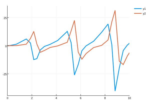
0.0 3.32215e-7 1.61467e-5 0.000580661 -16.7298 -9.02154 -6.25649then da is the timeseries for $\frac{\partial u(t)}{\partial p}$. We can plot this
using Plots
plot(sol.t,da',lw=3)
transposing so that the rows (the timeseries) is plotted.
For more information on the internal representation of the ODEForwardSensitivityProblem solution, see the direct forward sensitivity analysis manual page.
Example using adjoint_sensitivities for discrete adjoints
In this example we will show solving for the adjoint sensitivities of a discrete cost functional. First let's solve the ODE and get a high quality continuous solution:
function f(du,u,p,t)
  du[1] = dx = p[1]*u[1] - p[2]*u[1]*u[2]
  du[2] = dy = -p[3]*u[2] + u[1]*u[2]
end

p = [1.5,1.0,3.0]
prob = ODEProblem(f,[1.0;1.0],(0.0,10.0),p)
sol = solve(prob,Vern9(),abstol=1e-10,reltol=1e-10)
retcode: Success
Interpolation: specialized 9th order lazy interpolation
t: 90-element Vector{Float64}:
0.0
0.04354162443296621
0.12380859407417069
0.22510189540144385
0.3382985319836883
0.46890380279802657
0.6174892576286093
0.7793076265436987
0.9426296729311617
1.1035297132738715
⋮
9.244729158733456
9.335068756379858
9.415248631125761
9.50509929209238
9.597527812033242
9.701291332750895
9.821057116377693
9.944250653862317
10.0
u: 90-element Vector{Vector{Float64}}:
[1.0, 1.0]
[1.0238868996864754, 0.9170635457394599]
[1.0788467986761203, 0.7842060337333758]
[1.1683023062465243, 0.6483379638342583]
[1.295534400363908, 0.5305916985004335]
[1.480649833716726, 0.4296633117978187]
[1.746955109754463, 0.34941182084829564]
[2.1148147013059106, 0.29355585308179255]
[2.5825771410776186, 0.2635568268522404]
[3.153555478706522, 0.25761758045469585]
⋮
[1.6314661940676551, 3.8648589256063492]
[1.347246484276631, 3.368758570266105]
[1.180522294182296, 2.9296972074615564]
[1.0600968221501001, 2.4733351990986527]
[0.9880475912902639, 2.059772424016188]
[0.9520604797847954, 1.6679734411102043]
[0.9544648943647404, 1.304823279866495]
[0.9960140357940742, 1.0163902585048055]
[1.0263447674846644, 0.9096910781836495]Now let's calculate the sensitivity of the $\ell_2$ error against 1 at evenly spaced points in time, that is:
\[L(u,p,t)=\sum_{i=1}^{n}\frac{\Vert1-u(t_{i},p)\Vert^{2}}{2}\]
for $t_i = 0.5i$. This is the assumption that the data is data[i]=1.0. For this function, notice we have that:
\[\begin{aligned} dg_{1}&=1-u_{1} \\ dg_{2}&=1-u_{2} \\ & \quad \vdots \end{aligned}\]
and thus:
dg(out,u,p,t,i) = (out.=1.0.-u)dg (generic function with 1 method)Also, we can omit dgdp, because the cost function doesn't dependent on p. If we had data, we'd just replace 1.0 with data[i]. To get the adjoint sensitivities, call:
ts = 0:0.5:10
res = adjoint_sensitivities(sol,Vern9(),dg,ts,abstol=1e-14,
                            reltol=1e-14)
([-87.94877760334353, -22.488417339060884], [25.50065436691394 -77.25507872126092 93.53213951946763])This is super high accuracy. As always, there's a tradeoff between accuracy and computation time. We can check this almost exactly matches the autodifferentiation and numerical differentiation results:
using ForwardDiff,Calculus,ReverseDiff,Tracker
function G(p)
  tmp_prob = remake(prob,u0=convert.(eltype(p),prob.u0),p=p)
  sol = solve(tmp_prob,Vern9(),abstol=1e-14,reltol=1e-14,saveat=ts,
              sensealg=SensitivityADPassThrough())
  A = convert(Array,sol)
  sum(((1 .- A).^2)./2)
end
G([1.5,1.0,3.0])
res2 = ForwardDiff.gradient(G,[1.5,1.0,3.0])
res3 = Calculus.gradient(G,[1.5,1.0,3.0])
res4 = Tracker.gradient(G,[1.5,1.0,3.0])
res5 = ReverseDiff.gradient(G,[1.5,1.0,3.0])
3-element Vector{Float64}:
25.500637231791032
-77.25507741525361
93.53212756432536and see this gives the same values.