Solving Optimal Control Problems with Universal Differential Equations
Here we will solve a classic optimal control problem with a universal differential equation. Let
\[x^{′′} = u^3(t)\]
where we want to optimize our controller u(t) such that the following is minimized:
\[L(\theta) = \sum_i \Vert 4 - x(t_i) \Vert + 2 \Vert x^\prime(t_i) \Vert + \Vert u(t_i) \Vert\]
where $i$ is measured on (0,8) at 0.01 intervals. To do this, we rewrite the ODE in first order form:
\[\begin{aligned} x^\prime &= v \\ v^′ &= u^3(t) \\ \end{aligned}\]
and thus
\[L(\theta) = \sum_i \Vert 4 - x(t_i) \Vert + 2 \Vert v(t_i) \Vert + \Vert u(t_i) \Vert\]
is our loss function on the first order system. We thus choose a neural network form for $u$ and optimize the equation with respect to this loss. Note that we will first reduce control cost (the last term) by 10x in order to bump the network out of a local minimum. This looks like:
using Lux, DifferentialEquations, Optimization, OptimizationOptimJL, OptimizationFlux, Plots, Statistics, Random
rng = Random.default_rng()
tspan = (0.0f0,8.0f0)
ann = Lux.Chain(Lux.Dense(1,32,tanh), Lux.Dense(32,32,tanh), Lux.Dense(32,1))
θ, st = Lux.setup(rng, ann)
function dxdt_(dx,x,p,t)
    x1, x2 = x
    dx[1] = x[2]
    dx[2] = (ann([t],p,st)[1])[1]^3
end
x0 = [-4f0,0f0]
ts = Float32.(collect(0.0:0.01:tspan[2]))
prob = ODEProblem(dxdt_,x0,tspan,θ)
solve(prob,Vern9(),abstol=1e-10,reltol=1e-10)
function predict_adjoint(θ)
  Array(solve(prob,Vern9(),p=θ,saveat=ts,sensealg=InterpolatingAdjoint(autojacvec=ReverseDiffVJP(true))))
end
function loss_adjoint(θ)
  x = predict_adjoint(θ)
  mean(abs2,4.0 .- x[1,:]) + 2mean(abs2,x[2,:]) + mean(abs2,[first(ann([t],θ)) for t in ts])/10
end
l = loss_adjoint(θ)
callback = function (θ,l)
  println(l)
  p = plot(solve(remake(prob,p=θ),Tsit5(),saveat=0.01),ylim=(-6,6),lw=3)
  plot!(p,ts,[first(ann([t],θ)) for t in ts],label="u(t)",lw=3)
  display(p)
  return false
end
# Display the ODE with the current parameter values.
callback(θ,l)
loss1 = loss_adjoint(θ)
adtype = Optimization.AutoZygote()
optf = Optimization.OptimizationFunction((x,p)->loss_adjoint(x), adtype)

optprob = Optimization.OptimizationProblem(optf, θ)
res1 = Optimization.solve(optprob, ADAM(0.005), callback = callback,maxiters=100)

optprob2 = Optimization.OptimizationProblem(optf, res1.u)
res2 = Optimization.solve(optprob2,
                              BFGS(), maxiters=100,
                              allow_f_increases = false)
Now that the system is in a better behaved part of parameter space, we return to the original loss function to finish the optimization:
function loss_adjoint(θ)
x = predict_adjoint(θ)
mean(abs2,4.0 .- x[1,:]) + 2mean(abs2,x[2,:]) + mean(abs2,[first(ann([t],θ)) for t in ts])
end
optf3 = Optimization.OptimizationFunction((x,p)->loss_adjoint(x), adtype)
optprob3 = Optimization.OptimizationProblem(optf3, res2.u)
res3 = Optimization.solve(optprob3,
BFGS(),maxiters=100,
allow_f_increases = false)
l = loss_adjoint(res3.u)
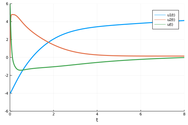
callback(res3.u,l)
p = plot(solve(remake(prob,p=res3.u),Tsit5(),saveat=0.01),ylim=(-6,6),lw=3)
plot!(p,ts,[first(ann([t],res3.u)) for t in ts],label="u(t)",lw=3)
savefig("optimal_control.png")