Direct Forward Sensitivity Analysis of ODEs

function ODEForwardSensitivityProblem(f::Union{Function,DiffEqBase.AbstractODEFunction}, u0,tspan,p=nothing, alg::AbstractForwardSensitivityAlgorithm = ForwardSensitivity(); kwargs...)

Local forward sensitivity analysis gives a solution along with a timeseries of the sensitivities. Thus if one wishes to have a derivative at every possible time point, directly using the ODEForwardSensitivityProblem can be the most efficient method.

ODEForwardSensitivityProblem Syntax

ODEForwardSensitivityProblem is similar to an ODEProblem, but takes an AbstractForwardSensitivityAlgorithm that describes how to append the forward sensitivity equation calculation to the time evolution to simultaneously compute the derivative of the solution with respect to parameters.

ODEForwardSensitivityProblem(f::SciMLBase.AbstractODEFunction,u0,
                             tspan,p=nothing,
                             sensealg::AbstractForwardSensitivityAlgorithm = ForwardSensitivity();
                             kwargs...)

Once constructed, this problem can be used in solve just like any other ODEProblem. The solution can be deconstructed into the ODE solution and sensitivities parts using the extract_local_sensitivities function, with the following dispatches:

extract_local_sensitivities(sol, asmatrix::Val=Val(false)) # Decompose the entire time series
extract_local_sensitivities(sol, i::Integer, asmatrix::Val=Val(false)) # Decompose sol[i]
extract_local_sensitivities(sol, t::Union{Number,AbstractVector}, asmatrix::Val=Val(false)) # Decompose sol(t)

For information on the mathematics behind these calculations, consult the sensitivity math page

Example using an ODEForwardSensitivityProblem

To define a sensitivity problem, simply use the ODEForwardSensitivityProblem type instead of an ODE type. For example, we generate an ODE with the sensitivity equations attached for the Lotka-Volterra equations by:

function f(du,u,p,t)
  du[1] = dx = p[1]*u[1] - p[2]*u[1]*u[2]
  du[2] = dy = -p[3]*u[2] + u[1]*u[2]
end

p = [1.5,1.0,3.0]
prob = ODEForwardSensitivityProblem(f,[1.0;1.0],(0.0,10.0),p)

This generates a problem which the ODE solvers can solve:

sol = solve(prob,DP8())

Note that the solution is the standard ODE system and the sensitivity system combined. We can use the following helper functions to extract the sensitivity information:

x,dp = extract_local_sensitivities(sol)
x,dp = extract_local_sensitivities(sol,i)
x,dp = extract_local_sensitivities(sol,t)

In each case, x is the ODE values and dp is the matrix of sensitivities The first gives the full timeseries of values and dp[i] contains the time series of the sensitivities of all components of the ODE with respect to ith parameter. The second returns the ith time step, while the third interpolates to calculate the sensitivities at time t. For example, if we do:

x,dp = extract_local_sensitivities(sol)
da = dp[1]

then da is the timeseries for $\frac{\partial u(t)}{\partial p}$. We can plot this

plot(sol.t,da',lw=3)

transposing so that the rows (the timeseries) is plotted.

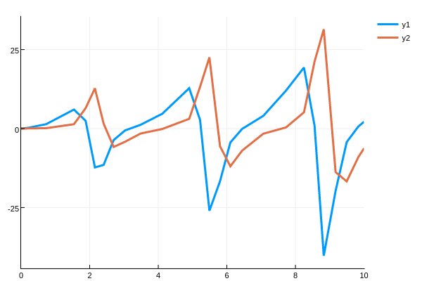
Here we see that there is a periodicity to the sensitivity which matches the periodicity of the Lotka-Volterra solutions. However, as time goes on the sensitivity increases. This matches the analysis of Wilkins in Sensitivity Analysis for Oscillating Dynamical Systems.

We can also quickly see that these values are equivalent to those given by automatic differentiation and numerical differentiation through the ODE solver:

using ForwardDiff, Calculus
function test_f(p)
  prob = ODEProblem(f,eltype(p).([1.0,1.0]),eltype(p).((0.0,10.0)),p)
  solve(prob,Vern9(),abstol=1e-14,reltol=1e-14,save_everystep=false)[end]
end

p = [1.5,1.0,3.0]
fd_res = ForwardDiff.jacobian(test_f,p)
calc_res = Calculus.finite_difference_jacobian(test_f,p)

Here we just checked the derivative at the end point.

Internal representation of the Solution

For completeness, we detail the internal representation. When using ForwardDiffSensitivity, the representation is with Dual numbers under the standard interpretation. The values for the ODE's solution at time i are the ForwardDiff.value.(sol[i]) portions, and the derivative with respect to parameter j is given by ForwardDiff.partials.(sol[i])[j].

When using ForwardSensitivity, the solution to the ODE are the first n components of the solution. This means we can grab the matrix of solution values like:

x = sol[1:sol.prob.indvars,:]

Since each sensitivity is a vector of derivatives for each function, the sensitivities are each of size sol.prob.indvars. We can pull out the parameter sensitivities from the solution as follows:

da = sol[sol.prob.indvars+1:sol.prob.indvars*2,:]
db = sol[sol.prob.indvars*2+1:sol.prob.indvars*3,:]
dc = sol[sol.prob.indvars*3+1:sol.prob.indvars*4,:]

This means that da[1,i] is the derivative of the x(t) by the parameter a at time sol.t[i]. Note that all of the functionality available to ODE solutions is available in this case, including interpolations and plot recipes (the recipes will plot the expanded system).

extractlocalsensitivities

Extracts the time series for the local sensitivities from the ODE solution. This requires that the ODE was defined via ODEForwardSensitivityProblem.

extract_local_sensitivities(sol, asmatrix::Val=Val(false)) # Decompose the entire time series
extract_local_sensitivities(sol, i::Integer, asmatrix::Val=Val(false)) # Decompose sol[i]
extract_local_sensitivities(sol, t::Union{Number,AbstractVector}, asmatrix::Val=Val(false)) # Decompose sol(t)