Bayesian Neural ODEs: NUTS
In this tutorial, we show how the DiffEqFlux.jl library in Julia can be seamlessly combined with Bayesian estimation libraries like AdvancedHMC.jl and Turing.jl. This enables converting Neural ODEs to Bayesian Neural ODEs, which enables us to estimate the error in the Neural ODE estimation and forecasting. In this tutorial, a working example of the Bayesian Neural ODE: NUTS sampler is shown.
For more details, please refer to Bayesian Neural Ordinary Differential Equations.
Copy-Pasteable Code
Before getting to the explanation, here's some code to start with. We will follow wil a full explanation of the definition and training process:
using DiffEqFlux, DifferentialEquations, Plots, AdvancedHMC, MCMCChains
using JLD, StatsPlots
u0 = [2.0; 0.0]
datasize = 40
tspan = (0.0, 1)
tsteps = range(tspan[1], tspan[2], length = datasize)
function trueODEfunc(du, u, p, t)
true_A = [-0.1 2.0; -2.0 -0.1]
du .= ((u.^3)'true_A)'
end
prob_trueode = ODEProblem(trueODEfunc, u0, tspan)
ode_data = Array(solve(prob_trueode, Tsit5(), saveat = tsteps))
dudt2 = FastChain((x, p) -> x.^3,
FastDense(2, 50, tanh),
FastDense(50, 2))
prob_neuralode = NeuralODE(dudt2, tspan, Tsit5(), saveat = tsteps)
function predict_neuralode(p)
Array(prob_neuralode(u0, p))
end
function loss_neuralode(p)
pred = predict_neuralode(p)
loss = sum(abs2, ode_data .- pred)
return loss, pred
end
l(θ) = -sum(abs2, ode_data .- predict_neuralode(θ)) - sum(θ .* θ)
function dldθ(θ)
x,lambda = Flux.Zygote.pullback(l,θ)
grad = first(lambda(1))
return x, grad
end
metric = DiagEuclideanMetric(length(prob_neuralode.p))
h = Hamiltonian(metric, l, dldθ)
integrator = Leapfrog(find_good_stepsize(h, Float64.(prob_neuralode.p)))
prop = AdvancedHMC.NUTS{MultinomialTS, GeneralisedNoUTurn}(integrator)
adaptor = StanHMCAdaptor(MassMatrixAdaptor(metric), StepSizeAdaptor(0.45, integrator))
samples, stats = sample(h, prop, Float64.(prob_neuralode.p), 500, adaptor, 500; progress=true)
losses = map(x-> x[1],[loss_neuralode(samples[i]) for i in 1:length(samples)])
##################### PLOTS: LOSSES ###############
scatter(losses, ylabel = "Loss", yscale= :log, label = "Architecture1: 500 warmup, 500 sample")
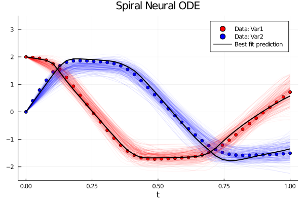
################### RETRODICTED PLOTS: TIME SERIES #################
pl = scatter(tsteps, ode_data[1,:], color = :red, label = "Data: Var1", xlabel = "t", title = "Spiral Neural ODE")
scatter!(tsteps, ode_data[2,:], color = :blue, label = "Data: Var2")
for k in 1:300
resol = predict_neuralode(samples[100:end][rand(1:400)])
plot!(tsteps,resol[1,:], alpha=0.04, color = :red, label = "")
plot!(tsteps,resol[2,:], alpha=0.04, color = :blue, label = "")
end
idx = findmin(losses)[2]
prediction = predict_neuralode(samples[idx])
plot!(tsteps,prediction[1,:], color = :black, w = 2, label = "")
plot!(tsteps,prediction[2,:], color = :black, w = 2, label = "Best fit prediction", ylims = (-2.5, 3.5))
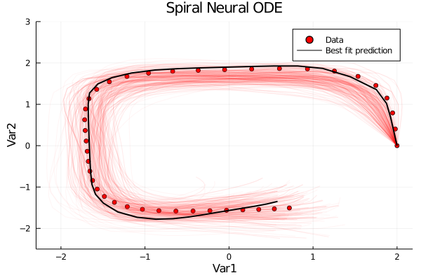
#################### RETRODICTED PLOTS - CONTOUR ####################
pl = scatter(ode_data[1,:], ode_data[2,:], color = :red, label = "Data", xlabel = "Var1", ylabel = "Var2", title = "Spiral Neural ODE")
for k in 1:300
resol = predict_neuralode(samples[100:end][rand(1:400)])
plot!(resol[1,:],resol[2,:], alpha=0.04, color = :red, label = "")
end
plot!(prediction[1,:], prediction[2,:], color = :black, w = 2, label = "Best fit prediction", ylims = (-2.5, 3))
Time Series Plots:
Contour Plots:
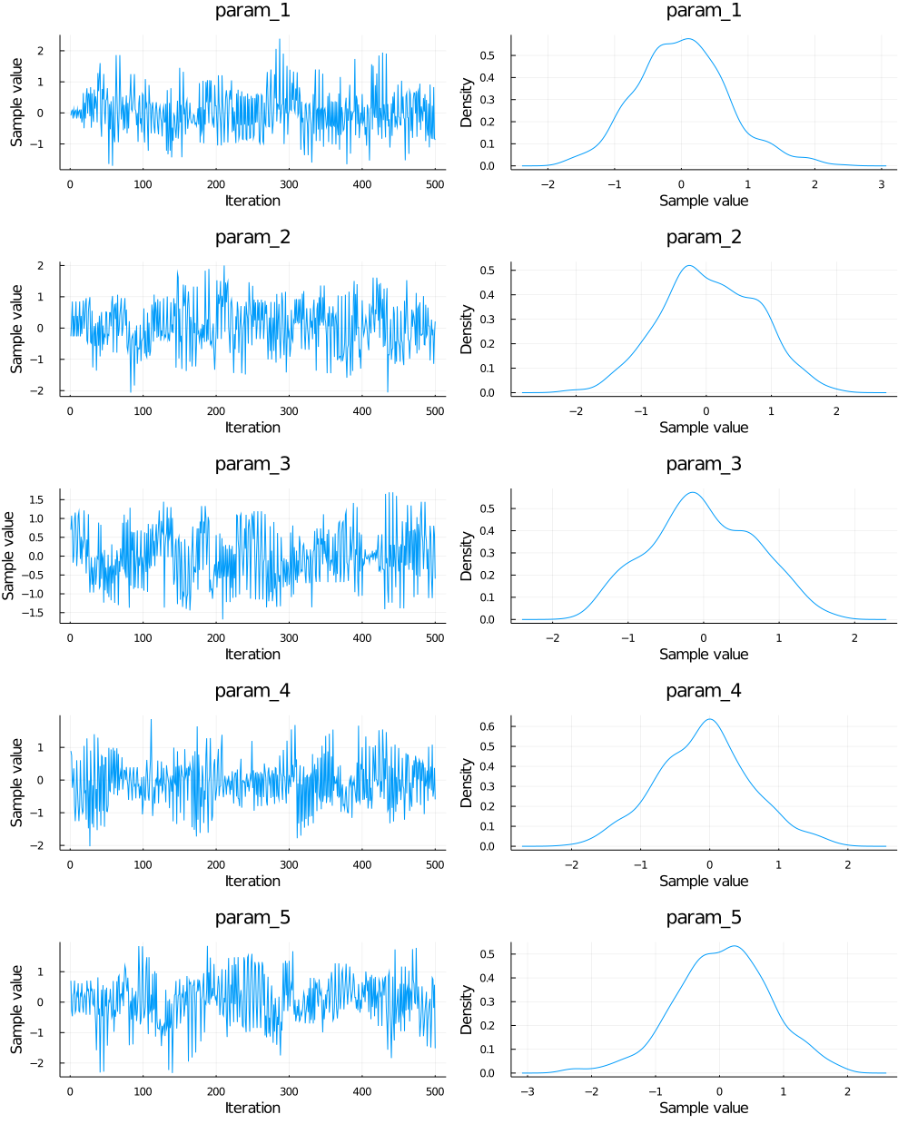
######################## CHAIN DIAGNOSIS PLOTS#########################
samples = hcat(samples...)
samples_reduced = samples[1:5, :]
samples_reshape = reshape(samples_reduced, (500, 5, 1))
Chain_Spiral = Chains(samples_reshape)
plot(Chain_Spiral)
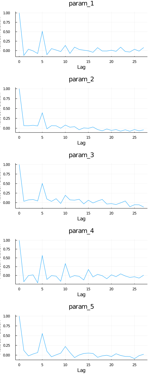
autocorplot(Chain_Spiral)
Chain Mixing Plot:
Auto-Correlation Plot:
Explanation
Step 1: Get the data from the Spiral ODE example
u0 = [2.0; 0.0]
datasize = 40
tspan = (0.0, 1)
tsteps = range(tspan[1], tspan[2], length = datasize)

function trueODEfunc(du, u, p, t)
    true_A = [-0.1 2.0; -2.0 -0.1]
    du .= ((u.^3)'true_A)'
end

prob_trueode = ODEProblem(trueODEfunc, u0, tspan)
ode_data = Array(solve(prob_trueode, Tsit5(), saveat = tsteps))
Step 2: Define the Neural ODE architecture.
Note that this step potentially offers a lot of flexibility in the number of layers/ number of units in each layer. It may not necessarily be true that a 100 units architecture is better at prediction/forecasting than a 50 unit architecture. On the other hand, a complicated architecture can take a huge computational time without increasing performance.
dudt2 = FastChain((x, p) -> x.^3,
                  FastDense(2, 50, tanh),
                  FastDense(50, 2))
prob_neuralode = NeuralODE(dudt2, tspan, Tsit5(), saveat = tsteps)
Step 3: Define the loss function for the Neural ODE.
function predict_neuralode(p)
    Array(prob_neuralode(u0, p))
end

function loss_neuralode(p)
    pred = predict_neuralode(p)
    loss = sum(abs2, ode_data .- pred)
    return loss, pred
end
Step 4: Now we start integrating the Bayesian estimation workflow as prescribed by the AdvancedHMC interface with the NeuralODE defined above.
The Advanced HMC interface requires us to specify: (a) the hamiltonian log density and its gradient , (b) the sampler and (c) the step size adaptor function.
For the hamiltonian log density, we use the loss function. The θ*θ term denotes the use of Gaussian priors.
The user can make several modifications to Step 4. The user can try different acceptance ratios, warmup samples and posterior samples. One can also use the Variational Inference (ADVI) framework, which doesn't work quite as well as NUTS. The SGLD (Stochastic Langevin Gradient Descent) sampler is seen to have a better performance than NUTS. Have a look at https://sebastiancallh.github.io/post/langevin/ for a quick introduction to SGLD.
l(θ) = -sum(abs2, ode_data .- predict_neuralode(θ)) - sum(θ .* θ)


function dldθ(θ)
    x,lambda = Flux.Zygote.pullback(l,θ)
    grad = first(lambda(1))
    return x, grad
end

metric  = DiagEuclideanMetric(length(prob_neuralode.p))

h = Hamiltonian(metric, l, dldθ)
We use the NUTS sampler with a acceptance ratio of δ= 0.45 in this example. In addition, we use Nesterov Dual Averaging for the Step Size adaptation.
We sample using 500 warmup samples and 500 posterior samples.
integrator = Leapfrog(find_good_stepsize(h, Float64.(prob_neuralode.p)))


prop = AdvancedHMC.NUTS{MultinomialTS, GeneralisedNoUTurn}(integrator)

adaptor = StanHMCAdaptor(MassMatrixAdaptor(metric), StepSizeAdaptor(0.45, integrator))

samples, stats = sample(h, prop, Float64.(prob_neuralode.p), 500, adaptor, 500; progress=true)
Step 5: Plot diagnostics.
A: Plot chain object and auto-correlation plot of the first 5 parameters.
samples = hcat(samples...)

samples_reduced = samples[1:5, :]

samples_reshape = reshape(samples_reduced, (500, 5, 1))

Chain_Spiral = Chains(samples_reshape)

plot(Chain_Spiral)

autocorplot(Chain_Spiral)
B: Plot retrodicted data.
####################TIME SERIES PLOTS###################
pl = scatter(tsteps, ode_data[1,:], color = :red, label = "Data: Var1", xlabel = "t", title = "Spiral Neural ODE")
scatter!(tsteps, ode_data[2,:], color = :blue, label = "Data: Var2")

for k in 1:300
    resol = predict_neuralode(samples[100:end][rand(1:400)])
    plot!(tsteps,resol[1,:], alpha=0.04, color = :red, label = "")
    plot!(tsteps,resol[2,:], alpha=0.04, color = :blue, label = "")
end

idx = findmin(losses)[2]
prediction = predict_neuralode(samples[idx])

plot!(tsteps,prediction[1,:], color = :black, w = 2, label = "")
plot!(tsteps,prediction[2,:], color = :black, w = 2, label = "Best fit prediction", ylims = (-2.5, 3.5))

####################CONTOUR PLOTS#########################3
pl = scatter(ode_data[1,:], ode_data[2,:], color = :red, label = "Data",  xlabel = "Var1", ylabel = "Var2", title = "Spiral Neural ODE")

for k in 1:300
    resol = predict_neuralode(samples[100:end][rand(1:400)])
    plot!(resol[1,:],resol[2,:], alpha=0.04, color = :red, label = "")
end

plot!(prediction[1,:], prediction[2,:], color = :black, w = 2, label = "Best fit prediction", ylims = (-2.5, 3))