Prediction error method (PEM)

When identifying linear systems from noisy data, the prediction-error method ^[Ljung] is close to a gold standard when it comes to the quality of the models it produces, but is also one of the computationally more expensive methods due to its reliance on iterative, gradient-based estimation. When we are identifying nonlinear models, we typically do not have the luxury of closed-form, non-iterative solutions, while PEM is easier to adopt to the nonlinear setting.^[Larsson]

Fundamentally, PEM changes the problem from minimizing a loss based on the simulation performance, to minimizing a loss based on shorter-term predictions. There are several benefits of doing so, and this example will highlight two:

• The loss is often easier to optimize.
• In addition to an accurate simulator, you also obtain a prediction for the system.
• With PEM, it's possible to estimate disturbance models.

The last point will not be illustrated in this tutorial, but we will briefly expand upon it here. Gaussian, zero-mean measurement noise is usually not very hard to handle. Disturbances that affect the state of the system may, however, cause all sorts of havoc on the estimate. Consider wind affecting an aircraft, deriving a statistical and dynamical model of the wind may be doable, but unless you measure the exact wind affecting the aircraft, making use of the model during parameter estimation is impossible. The wind is an unmeasured load disturbance that affects the state of the system through its own dynamics model. Using the techniques illustrated in this tutorial, it's possible to estimate the influence of the wind during the experiment that generated the data and reduce or eliminate the bias it otherwise causes in the parameter estimates.

We will start by illustrating a common problem with simulation-error minimization. Imagine a pendulum with unknown length that is to be estimated. A small error in the pendulum length causes the frequency of oscillation to change. Over sufficiently large horizon, two sinusoidal signals with different frequencies become close to orthogonal to each other. If some form of squared-error loss is used, the loss landscape will be horribly non-convex in this case, indeed, we will illustrate exactly this below.

Another case that poses a problem for simulation-error estimation is when the system is unstable or chaotic. A small error in either the initial condition or the parameters may cause the simulation error to diverge and its gradient to become meaningless.

In both of these examples, we may make use of measurements we have of the evolution of the system to prevent the simulation error from diverging. For instance, if we have measured the angle of the pendulum, we can make use of this measurement to adjust the angle during the simulation to make sure it stays close to the measured angle. Instead of performing a pure simulation, we instead say that we predict the state a while forward in time, given all the measurements up until the current time point. By minimizing this prediction rather than the pure simulation, we can often prevent the model error from diverging even though we have a poor initial guess.

We start by defining a model of the pendulum. The model takes a parameter $L$ corresponding to the length of the pendulum.

using DifferentialEquations, Optimization, OptimizationOptimJL, OptimizationPolyalgorithms, Plots, Statistics, DataInterpolations, ForwardDiff

tspan = (0.1f0, Float32(20.0))
tsteps = range(tspan[1], tspan[2], length = 1000)

u0 = [0f0, 3f0] # Initial angle and angular velocity

function simulator(du,u,p,t) # Pendulum dynamics
    g = 9.82f0 # Gravitational constant
    L = p isa Number ? p : p[1] # Length of the pendulum
    gL = g/L
    θ  = u[1]
    dθ = u[2]
    du[1] = dθ
    du[2] = -gL * sin(θ)
end

We assume that the true length of the pendulum is $L = 1$, and generate some data from this system.

prob = ODEProblem(simulator,u0,tspan,1.0) # Simulate with L = 1
sol = solve(prob, Tsit5(), saveat=tsteps, abstol = 1e-8, reltol = 1e-6)
y = sol[1,:] # This is the data we have available for parameter estimation
plot(y, title="Pendulum simulation", label="angle")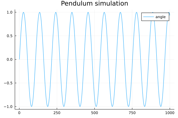

We also define functions that simulate the system and calculate the loss, given a parameter p corresponding to the length.

function simulate(p)
    _prob = remake(prob,p=p)
    solve(_prob, Tsit5(), saveat=tsteps, abstol = 1e-8, reltol = 1e-6)[1,:]
end

function simloss(p)
    yh = simulate(p)
    e2 = yh
    e2 .= abs2.(y .- yh)
    return mean(e2)
end

We now look at the loss landscape as a function of the pendulum length:

Ls = 0.01:0.01:2
simlosses = simloss.(Ls)
fig_loss = plot(Ls, simlosses, title = "Loss landscape", xlabel="Pendulum length", ylabel = "MSE loss", lab="Simulation loss")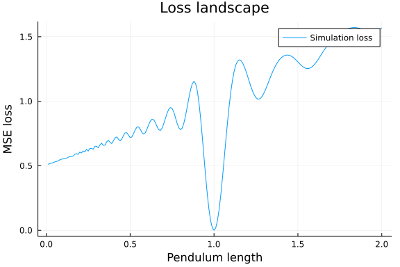

This figure is interesting, the loss is of course 0 for the true value $L=1$, but for values $L < 1$, the overall slope actually points in the wrong direction! Moreover, the loss is oscillatory, indicating that this is a terrible function to optimize, and that we would need a very good initial guess for a local search to converge to the true value. Note, this example is chosen to be one-dimensional in order to allow these kinds of visualizations, and one-dimensional problems are typically not hard to solve, but the reasoning extends to higher-dimensional and harder problems.

We will now move on to defining a predictor model. Our predictor will be very simple, each time step, we will calculate the error $e$ between the simulated angle $\theta$ and the measured angle $y$. A part of this error will be used to correct the state of the pendulum. The correction we use is linear and looks like $Ke = K(y - \theta)$. We have formed what is commonly referred to as a (linear) observer. The Kalman filter is a particular kind of linear observer, where $K$ is calculated based on a statistical model of the disturbances that act on the system. We will stay with a simple, fixed-gain observer here for simplicity.

To feed the sampled data into the continuous-time simulation, we make use of an interpolator. We also define new functions, predictor that contains the pendulum dynamics with the observer correction, a prediction function that performs the rollout (we're not using the word simulation to not confuse with the setting above) and a loss function.

y_int = LinearInterpolation(y,tsteps)

function predictor(du,u,p,t)
    g = 9.82f0
    L, K, y = p # pendulum length, observer gain and measurements
    gL = g/L
    θ  = u[1]
    dθ = u[2]
    yt = y(t)
    e = yt - θ
    du[1] = dθ + K*e
    du[2] = -gL * sin(θ) 
end

predprob = ODEProblem(predictor,u0,tspan,nothing)

function prediction(p)
    p_full = (p..., y_int)
    _prob = remake(predprob,u0=eltype(p_full).(u0),p=p_full)
    solve(_prob, Tsit5(), saveat=tsteps, abstol = 1e-8, reltol = 1e-6)[1,:]
end

function predloss(p)
    yh = prediction(p)
    e2 = yh
    e2 .= abs2.(y .- yh)
    return mean(e2)
end

predlosses = map(Ls) do L
    p = (L, 1) # use K = 1
    predloss(p)
end

plot!(Ls, predlosses, lab="Prediction loss")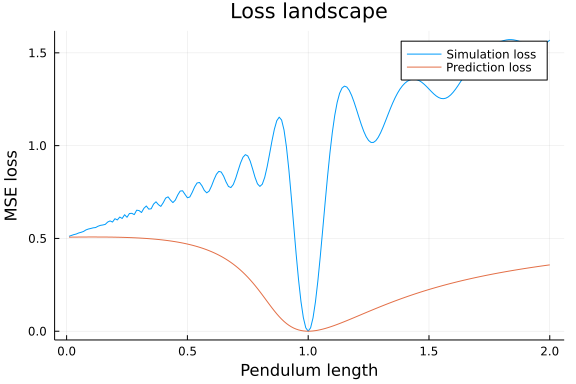

Once gain we look at the loss as a function of the parameter, and this time it looks a lot better. The loss is not convex, but the gradient points in the right direction over a much larger interval. Here, we arbitrarily set the observer gain to $K=1$, we will later let the optimizer learn this parameter.

For completeness, we also perform estimation using both losses. We choose an initial guess we know will be hard for the simulation-error minimization just to drive home the point:

L0 = [0.7] # Initial guess of pendulum length
adtype = Optimization.AutoForwardDiff()
optf = Optimization.OptimizationFunction((x,p)->simloss(x), adtype)
optprob = Optimization.OptimizationProblem(optf, L0)

ressim = Optimization.solve(optprob, PolyOpt(),
                                    maxiters = 5000)
ysim = simulate(ressim.u)

plot(tsteps, [y ysim], label=["Data" "Simulation model"])

p0 = [0.7, 1.0] # Initial guess of length and observer gain K
optf2 = Optimization.OptimizationFunction((p,_)->predloss(p), adtype)
optfunc2 = Optimization.instantiate_function(optf2, p0, adtype, nothing)
optprob2 = Optimization.OptimizationProblem(optfunc2, p0)

respred = Optimization.solve(optprob2, PolyOpt(),
                                    maxiters = 5000)
ypred = simulate(respred.u)

plot!(tsteps, ypred, label="Prediction model")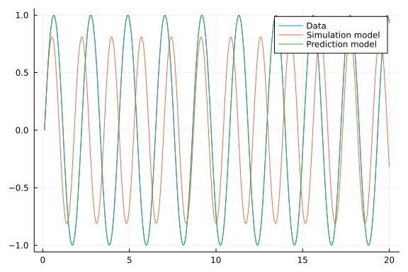

The estimated parameters $(L, K)$ are

respred.u

Now, we might ask ourselves why we used a correct on the form $Ke$ and didn't instead set the angle in the simulation equal to the measurement. The reason is twofold

1. If our prediction of the angle is 100% based on the measurements, the model parameters do not matter for the prediction and we can thus not hope to learn their values.
2. The measurement is usually noisy, and we thus want to fuse the predictive power of the model with the information of the measurements. The Kalman filter is an optimal approach to this information fusion under special circumstances (linear model, Gaussian noise).

We thus let the optimization learn the best value of the observer gain in order to make the best predictions.

As a last step, we perform the estimation also with some measurement noise to verify that it does something reasonable:

yn = y .+ 0.1f0 .* randn.(Float32)
y_int = LinearInterpolation(yn,tsteps) # redefine the interpolator to contain noisy measurements

optf = Optimization.OptimizationFunction((x,p)->predloss(x), adtype)
optprob = Optimization.OptimizationProblem(optf, p0)

resprednoise = Optimization.solve(optprob, PolyOpt(),
                                    maxiters = 5000)

yprednoise = prediction(resprednoise.u)
plot!(tsteps, yprednoise, label="Prediction model with noisy measurements")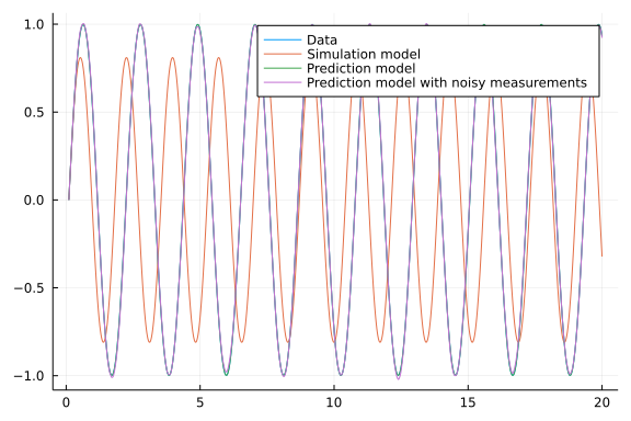

resprednoise.u

This example has illustrated basic use of the prediction-error method for parameter estimation. In our example, the measurement we had corresponded directly to one of the states, and coming up with an observer/predictor that worked was not too hard. For more difficult cases, we may opt to use a nonlinear observer, such as an extended Kalman filter (EKF) or design a Kalman filter based on a linearization of the system around some operating point.

As a last note, there are several other methods available to improve the loss landscape and avoid local minima, such as multiple-shooting. The prediction-error method can easily be combined with most of those methods.

References: