Optimization of Stochastic Differential Equations
Here we demonstrate sensealg = ForwardDiffSensitivity() (provided by DiffEqSensitivity.jl) for forward-mode automatic differentiation of a small stochastic differential equation. For large parameter equations, like neural stochastic differential equations, you should use reverse-mode automatic differentiation. However, forward-mode can be more efficient for low numbers of parameters (<100). (Note: the default is reverse-mode AD which is more suitable for things like neural SDEs!)
Example 1: Fitting Data with SDEs via Method of Moments and Parallelism
Let's do the most common scenario: fitting data. Let's say our ecological system is a stochastic process. Each time we solve this equation we get a different solution, so we need a sensible data source.
using DiffEqFlux, DifferentialEquations, Plots
function lotka_volterra!(du,u,p,t)
  x,y = u
  α,β,γ,δ = p
  du[1] = dx = α*x - β*x*y
  du[2] = dy = δ*x*y - γ*y
end
u0 = [1.0,1.0]
tspan = (0.0,10.0)

function multiplicative_noise!(du,u,p,t)
  x,y = u
  du[1] = p[5]*x
  du[2] = p[6]*y
end
p = [1.5,1.0,3.0,1.0,0.3,0.3]

prob = SDEProblem(lotka_volterra!,multiplicative_noise!,u0,tspan,p)
sol = solve(prob)
plot(sol)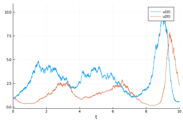
Let's assume that we are observing the seasonal behavior of this system and have 10,000 years of data, corresponding to 10,000 observations of this timeseries. We can utilize this to get the seasonal means and variances. To simulate that scenario, we will generate 10,000 trajectories from the SDE to build our dataset:
using Statistics
ensembleprob = EnsembleProblem(prob)
@time sol = solve(ensembleprob,SOSRI(),saveat=0.1,trajectories=10_000)
truemean = mean(sol,dims=3)[:,:]
truevar  = var(sol,dims=3)[:,:]
From here, we wish to utilize the method of moments to fit the SDE's parameters. Thus our loss function will be to solve the SDE a bunch of times and compute moment equations and use these as our loss against the original series. We then plot the evolution of the means and variances to verify the fit. For example:
function loss(p)
tmp_prob = remake(prob,p=p)
ensembleprob = EnsembleProblem(tmp_prob)
tmp_sol = solve(ensembleprob,SOSRI(),saveat=0.1,trajectories=1000)
arrsol = Array(tmp_sol)
sum(abs2,truemean - mean(arrsol,dims=3)) + 0.1sum(abs2,truevar - var(arrsol,dims=3)),arrsol
end
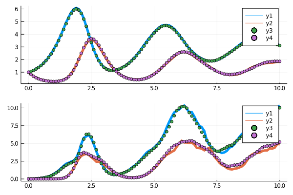
function cb2(p,l,arrsol)
@show p,l
means = mean(arrsol,dims=3)[:,:]
vars = var(arrsol,dims=3)[:,:]
p1 = plot(sol[1].t,means',lw=5)
scatter!(p1,sol[1].t,truemean')
p2 = plot(sol[1].t,vars',lw=5)
scatter!(p2,sol[1].t,truevar')
p = plot(p1,p2,layout = (2,1))
display(p)
false
endWe can then use Optimization.solve to fit the SDE:
using Optimization, OptimizationOptimJL
pinit = [1.2,0.8,2.5,0.8,0.1,0.1]
adtype = Optimization.AutoZygote()
optf = Optimization.OptimizationFunction((x,p) -> loss(x), adtype)
optprob = Optimization.OptimizationProblem(optf, pinit)
@time res = Optimization.solve(optprob,ADAM(0.05),callback=cb2,maxiters = 100)
The final print out was:
(p, l) = ([1.5242134195974462, 1.019859938499017, 2.9120928257869227, 0.9840408090733335, 0.29427123791721765, 0.3334393815923646], 1.7046719990657184)Notice that both the parameters of the deterministic drift equations and the stochastic portion (the diffusion equation) are fit through this process! Also notice that the final fit of the moment equations is close:
The time for the full fitting process was:
250.654845 seconds (4.69 G allocations: 104.868 GiB, 11.87% gc time)approximately 4 minutes.
Example 2: Fitting SDEs via Bayesian Quasi-Likelihood Approaches
An inference method which can be much more efficient in many cases is the quasi-likelihood approach. This approach matches the random likelihood of the SDE output with the random sampling of a Bayesian inference problem to more efficiently directly estimate the posterior distribution. For more information, please see the Turing.jl Bayesian Differential Equations tutorial
Example 3: Controlling SDEs to an objective
In this example, we will find the parameters of the SDE that force the solution to be close to the constant 1.
using DifferentialEquations, DiffEqFlux, Optimization, OptimizationJL, Plots

function lotka_volterra!(du, u, p, t)
  x, y = u
  α, β, δ, γ = p
  du[1] = dx = α*x - β*x*y
  du[2] = dy = -δ*y + γ*x*y
end

function lotka_volterra_noise!(du, u, p, t)
  du[1] = 0.1u[1]
  du[2] = 0.1u[2]
end

u0 = [1.0,1.0]
tspan = (0.0, 10.0)
p = [2.2, 1.0, 2.0, 0.4]
prob_sde = SDEProblem(lotka_volterra!, lotka_volterra_noise!, u0, tspan)


function predict_sde(p)
  return Array(solve(prob_sde, SOSRI(), p=p,
               sensealg = ForwardDiffSensitivity(), saveat = 0.1))
end

loss_sde(p) = sum(abs2, x-1 for x in predict_sde(p))
For this training process, because the loss function is stochastic, we will use the ADAM optimizer from Flux.jl. The Optimization.solve function is the same as before. However, to speed up the training process, we will use a global counter so that way we only plot the current results every 10 iterations. This looks like:
callback = function (p, l)
  display(l)
  remade_solution = solve(remake(prob_sde, p = p), SOSRI(), saveat = 0.1)
  plt = plot(remade_solution, ylim = (0, 6))
  display(plt)
  return false
end
Let's optimize
adtype = Optimization.AutoZygote()
optf = Optimization.OptimizationFunction((x,p) -> loss_sde(x), adtype)

optprob = Optimization.OptimizationProblem(optf, p)
result_sde = Optimization.solve(optprob, ADAM(0.1),
                                    callback = callback, maxiters = 100)