Neural Stochastic Differential Equations

With neural stochastic differential equations, there is once again a helper form neural_dmsde which can be used for the multiplicative noise case (consult the layers API documentation, or this full example using the layer function).

However, since there are far too many possible combinations for the API to support, in many cases you will want to performantly define neural differential equations for non-ODE systems from scratch. For these systems, it is generally best to use TrackerAdjoint with non-mutating (out-of-place) forms. For example, the following defines a neural SDE with neural networks for both the drift and diffusion terms:

dudt(u, p, t) = model(u)
g(u, p, t) = model2(u)
prob = SDEProblem(dudt, g, x, tspan, nothing)

where model and model2 are different neural networks. The same can apply to a neural delay differential equation. Its out-of-place formulation is f(u,h,p,t). Thus for example, if we want to define a neural delay differential equation which uses the history value at p.tau in the past, we can define:

dudt!(u, h, p, t) = model([u; h(t - p.tau)])
prob = DDEProblem(dudt_, u0, h, tspan, nothing)

First let's build training data from the same example as the neural ODE:

using Plots, Statistics
using Lux, Optimization, OptimizationFlux, DiffEqFlux, StochasticDiffEq, DiffEqBase.EnsembleAnalysis, Random

rng = Random.default_rng()
u0 = Float32[2.; 0.]
datasize = 30
tspan = (0.0f0, 1.0f0)
tsteps = range(tspan[1], tspan[2], length = datasize)

function trueSDEfunc(du, u, p, t)
    true_A = [-0.1 2.0; -2.0 -0.1]
    du .= ((u.^3)'true_A)'
end

mp = Float32[0.2, 0.2]
function true_noise_func(du, u, p, t)
    du .= mp.*u
end

prob_truesde = SDEProblem(trueSDEfunc, true_noise_func, u0, tspan)

For our dataset we will use DifferentialEquations.jl's parallel ensemble interface to generate data from the average of 10,000 runs of the SDE:

# Take a typical sample from the mean
ensemble_prob = EnsembleProblem(prob_truesde)
ensemble_sol = solve(ensemble_prob, SOSRI(), trajectories = 10000)
ensemble_sum = EnsembleSummary(ensemble_sol)

sde_data, sde_data_vars = Array.(timeseries_point_meanvar(ensemble_sol, tsteps))

Now we build a neural SDE. For simplicity we will use the NeuralDSDE neural SDE with diagonal noise layer function:

drift_dudt = Lux.Chain(ActivationFunction(x -> x.^3),
                       Lux.Dense(2, 50, tanh),
                       Lux.Dense(50, 2))
p1, st1 = Lux.setup(rng, drift_dudt)

diffusion_dudt = Lux.Chain(Lux.Dense(2, 2))
p2, st2 = Lux.setup(rng, diffusion_dudt)

p1 = Lux.ComponentArray(p1)
p2 = Lux.ComponentArray(p2)
#Component Arrays doesn't provide a name to the first ComponentVector, only subsequent ones get a name for dereferencing
p = [p1, p2]

neuralsde = NeuralDSDE(drift_dudt, diffusion_dudt, tspan, SOSRI(),
                       saveat = tsteps, reltol = 1e-1, abstol = 1e-1)

Let's see what that looks like:

# Get the prediction using the correct initial condition
prediction0, st1, st2 = neuralsde(u0,p,st1,st2)

drift_(u, p, t) = drift_dudt(u, p[1], st1)[1]
diffusion_(u, p, t) = diffusion_dudt(u, p[2], st2)[1]

prob_neuralsde = SDEProblem(drift_, diffusion_, u0,(0.0f0, 1.2f0), p)

ensemble_nprob = EnsembleProblem(prob_neuralsde)
ensemble_nsol = solve(ensemble_nprob, SOSRI(), trajectories = 100,
                      saveat = tsteps)
ensemble_nsum = EnsembleSummary(ensemble_nsol)

plt1 = plot(ensemble_nsum, title = "Neural SDE: Before Training")
scatter!(plt1, tsteps, sde_data', lw = 3)

scatter(tsteps, sde_data[1,:], label = "data")
scatter!(tsteps, prediction0[1,:], label = "prediction")

Now just as with the neural ODE we define a loss function that calculates the mean and variance from n runs at each time point and uses the distance from the data values:

function predict_neuralsde(p, u = u0)
  return Array(neuralsde(u, p, st1, st2)[1])
end

function loss_neuralsde(p; n = 100)
  u = repeat(reshape(u0, :, 1), 1, n)
  samples = predict_neuralsde(p, u)
  means = mean(samples, dims = 2)
  vars = var(samples, dims = 2, mean = means)[:, 1, :]
  means = means[:, 1, :]
  loss = sum(abs2, sde_data - means) + sum(abs2, sde_data_vars - vars)
  return loss, means, vars
end

list_plots = []
iter = 0

# Callback function to observe training
callback = function (p, loss, means, vars; doplot = false)
  global list_plots, iter

  if iter == 0
    list_plots = []
  end
  iter += 1

  # loss against current data
  display(loss)

  # plot current prediction against data
  plt = Plots.scatter(tsteps, sde_data[1,:], yerror = sde_data_vars[1,:],
                     ylim = (-4.0, 8.0), label = "data")
  Plots.scatter!(plt, tsteps, means[1,:], ribbon = vars[1,:], label = "prediction")
  push!(list_plots, plt)

  if doplot
    display(plt)
  end
  return false
end

Now we train using this loss function. We can pre-train a little bit using a smaller n and then decrease it after it has had some time to adjust towards the right mean behavior:

opt = ADAM(0.025)

# First round of training with n = 10
adtype = Optimization.AutoZygote()
optf = Optimization.OptimizationFunction((x,p) -> loss_neuralsde(x, n=10), adtype)
optprob = Optimization.OptimizationProblem(optf, p)
result1 = Optimization.solve(optprob, opt,
                                 callback = callback, maxiters = 100)

We resume the training with a larger n. (WARNING - this step is a couple of orders of magnitude longer than the previous one).

optf2 = Optimization.OptimizationFunction((x,p) -> loss_neuralsde(x, n=100), adtype)
optprob2 = Optimization.OptimizationProblem(optf2, result1.u)
result2 = Optimization.solve(optprob2, opt,
                                 callback = callback, maxiters = 100)

And now we plot the solution to an ensemble of the trained neural SDE:

_, means, vars = loss_neuralsde(result2.u, n = 1000)

plt2 = Plots.scatter(tsteps, sde_data', yerror = sde_data_vars',
                     label = "data", title = "Neural SDE: After Training",
                     xlabel = "Time")
plot!(plt2, tsteps, means', lw = 8, ribbon = vars', label = "prediction")

plt = plot(plt1, plt2, layout = (2, 1))
savefig(plt, "NN_sde_combined.png"); nothing # sde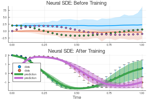

Try this with GPUs as well!