Bayesian Neural ODEs: SGLD
Recently, Neural Ordinary Differential Equations has emerged as a powerful framework for modeling physical simulations without explicitly defining the ODEs governing the system, but learning them via machine learning. However, the question: Can Bayesian learning frameworks be integrated with Neural ODEs to robustly quantify the uncertainty in the weights of a Neural ODE? remains unanswered.
In this tutorial, a working example of the Bayesian Neural ODE: SGLD sampler is shown. SGLD stands for Stochastic Langevin Gradient Descent.
For an introduction to SGLD, please refer to Introduction to SGLD in Julia
For more details regarding Bayesian Neural ODEs, please refer to Bayesian Neural Ordinary Differential Equations.
Copy-Pasteable Code
Before getting to the explanation, here's some code to start with. We will follow with a full explanation of the definition and training process:
using DiffEqFlux, DifferentialEquations, Flux
using Plots, StatsPlots
u0 = Float32[1., 1.]
p = [1.5, 1., 3., 1.]
datasize = 45
tspan = (0.0f0, 14.f0)
tsteps = tspan[1]:0.1:tspan[2]
function lv(u, p, t)
x, y = u
α, β, γ, δ = p
dx = α*x - β*x*y
dy = δ*x*y - γ*y
du = [dx, dy]
end
trueodeprob = ODEProblem(lv, u0, tspan, p)
ode_data = Array(solve(trueodeprob, Tsit5(), saveat = tsteps))
y_train = ode_data[:, 1:35]
dudt = FastChain(FastDense(2, 50, tanh), FastDense(50, 2))
prob_node = NeuralODE(dudt, (0., 14.), Tsit5(), saveat = tsteps)
train_prob = NeuralODE(dudt, (0., 3.5), Tsit5(), saveat = tsteps[1:35])
function predict(p)
Array(train_prob(u0, p))
end
function loss(p)
sum(abs2, y_train .- predict(p))
end
sgld(∇L, θᵢ, t, a = 2.5e-3, b = 0.05, γ = 0.35) = begin
ϵ = a*(b + t)^-γ
η = ϵ.*randn(size(θᵢ))
Δθᵢ = .5ϵ*∇L + η
θᵢ .-= Δθᵢ
end
parameters = []
losses = Float64[]
grad_norm = Float64[]
θ = deepcopy(prob_node.p)
@time for t in 1:45000
grad = gradient(loss, θ)[1]
sgld(grad, θ, t)
tmp = deepcopy(θ)
append!(losses, loss(θ))
append!(grad_norm, sum(abs2, grad))
append!(parameters, [tmp])
println(loss(θ))
end
plot(losses, yscale = :log10)
plot(grad_norm, yscale =:log10)
using StatsPlots
sampled_par = parameters[43000: 45000]
##################### PLOTS: LOSSES ###############
sampled_loss = [loss(p) for p in sampled_par]
density(sampled_loss)
#################### RETRODICTED PLOTS - TIME SERIES AND CONTOUR PLOTS ####################
_, i_min = findmin(sampled_loss)
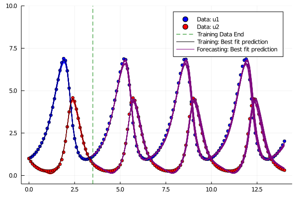
plt = scatter(tsteps,ode_data[1,:], colour = :blue, label = "Data: u1", ylim = (-.5, 10.))
scatter!(plt, tsteps, ode_data[2,:], colour = :red, label = "Data: u2")
phase_plt = scatter(ode_data[1,:], ode_data[2,:], colour = :red, label = "Data", xlim = (-.25, 7.), ylim = (-2., 6.5))
for p in sampled_par
s = prob_node(u0, p)
plot!(plt, tsteps[1:35], s[1,1:35], colour = :blue, lalpha = 0.04, label =:none)
plot!(plt, tsteps[35:end], s[1, 35:end], colour =:purple, lalpha = 0.04, label =:none)
plot!(plt, tsteps[1:35], s[2,1:35], colour = :red, lalpha = 0.04, label=:none)
plot!(plt, tsteps[35:end], s[2,35:end], colour = :purple, lalpha = 0.04, label=:none)
plot!(phase_plt, s[1,1:35], s[2,1:35], colour =:red, lalpha = 0.04, label=:none)
plot!(phase_plt, s[1,35:end], s[2, 35:end], colour = :purple, lalpha = 0.04, label=:none)
end
plt
phase_plt
plot!(plt, [3.5], seriestype =:vline, colour = :green, linestyle =:dash,label = "Training Data End")
bestfit = prob_node(u0, sampled_par[i_min])
plot(bestfit)
plot!(plt, tsteps[1:35], bestfit[2, 1:35], colour =:black, label = "Training: Best fit prediction")
plot!(plt, tsteps[35:end], bestfit[2, 35:end], colour =:purple, label = "Forecasting: Best fit prediction")
plot!(plt, tsteps[1:35], bestfit[1, 1:35], colour =:black, label = :none)
plot!(plt, tsteps[35:end], bestfit[1, 35:end], colour =:purple, label = :none)
plot!(phase_plt,bestfit[1,1:40], bestfit[2, 1:40], colour = :black, label = "Training: Best fit prediction")
plot!(phase_plt,bestfit[1, 40:end], bestfit[2, 40:end], colour = :purple, label = "Forecasting: Best fit prediction")
savefig(plt, "C:/Users/16174/Desktop/Julia Lab/MSML2021/BayesianNODE_SGLD_Plot1.png")
savefig(phase_plt, "C:/Users/16174/Desktop/Julia Lab/MSML2021/BayesianNODE_SGLD_Plot2.png")
Time Series Plots:
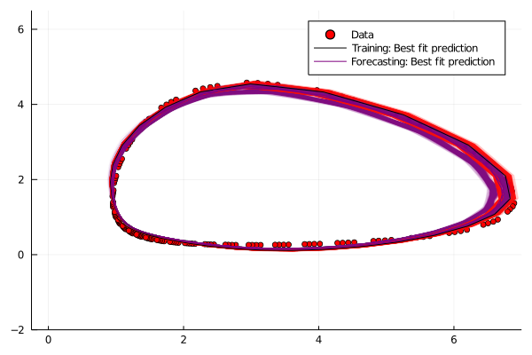
Contour Plots:
Explanation
Step1: Get the data from the Lotka Volterra ODE example
u0 = Float32[1., 1.]
p = [1.5, 1., 3., 1.]
datasize = 45
tspan = (0.0f0, 14.f0)
tsteps = tspan[1]:0.1:tspan[2]

function lv(u, p, t)
    x, y = u
    α, β, γ, δ = p
    dx = α*x - β*x*y
    dy = δ*x*y - γ*y
    du = [dx, dy]
end

trueodeprob = ODEProblem(lv, u0, tspan, p)
ode_data = Array(solve(trueodeprob, Tsit5(), saveat = tsteps))
y_train = ode_data[:, 1:35]
Step2: Define the Neural ODE architecture. Note that this step potentially offers a lot of flexibility in the number of layers/ number of units in each layer.
dudt = FastChain(FastDense(2, 50, tanh), FastDense(50, 2))
prob_node = NeuralODE(dudt, (0., 14.), Tsit5(), saveat = tsteps)
train_prob = NeuralODE(dudt, (0., 3.5), Tsit5(), saveat = tsteps[1:35])
Step3: Define the loss function for the Neural ODE.
function predict(p)
    Array(train_prob(u0, p))
end

function loss(p)
    sum(abs2, y_train .- predict(p))
end
Step4: Now we start integrating the Stochastic Langevin Gradient Descent(SGLD) framework.
The SGLD (Stochastic Langevin Gradient Descent) sampler is seen to have a better performance than NUTS whose tutorial is also shown in a separate document. Have a look at https://sebastiancallh.github.io/post/langevin/ for a quick introduction to SGLD.
Note that we sample from the last 2000 iterations.
sgld(∇L, θᵢ, t, a = 2.5e-3, b = 0.05, γ = 0.35) = begin
    ϵ = a*(b + t)^-γ
    η = ϵ.*randn(size(θᵢ))
    Δθᵢ = .5ϵ*∇L + η
    θᵢ .-= Δθᵢ
end

parameters = []
losses = Float64[]
grad_norm = Float64[]

θ = deepcopy(prob_node.p)
@time for t in 1:45000
    grad = gradient(loss, θ)[1]
    sgld(grad, θ, t)
    tmp = deepcopy(θ)
    append!(losses, loss(θ))
    append!(grad_norm, sum(abs2, grad))
    append!(parameters, [tmp])
    println(loss(θ))
end
plot(losses, yscale = :log10)
plot(grad_norm, yscale =:log10)

using StatsPlots
sampled_par = parameters[43000: 45000]
Step5: Plot Retrodicted Plots (Estimation and Forecasting).
################### RETRODICTED PLOTS - TIME SERIES AND CONTOUR PLOTS ####################

_, i_min = findmin(sampled_loss)

plt = scatter(tsteps,ode_data[1,:], colour = :blue, label = "Data: u1", ylim = (-.5, 10.))
scatter!(plt, tsteps, ode_data[2,:], colour = :red, label = "Data: u2")
phase_plt = scatter(ode_data[1,:], ode_data[2,:], colour = :red, label = "Data", xlim = (-.25, 7.), ylim = (-2., 6.5))

for p in sampled_par
    s = prob_node(u0, p)
    plot!(plt, tsteps[1:35], s[1,1:35], colour = :blue, lalpha = 0.04, label =:none)
    plot!(plt, tsteps[35:end], s[1, 35:end], colour =:purple, lalpha = 0.04, label =:none)
    plot!(plt, tsteps[1:35], s[2,1:35], colour = :red, lalpha = 0.04, label=:none)
    plot!(plt, tsteps[35:end], s[2,35:end], colour = :purple, lalpha = 0.04, label=:none)
    plot!(phase_plt, s[1,1:35], s[2,1:35], colour =:red, lalpha = 0.04, label=:none)
    plot!(phase_plt, s[1,35:end], s[2, 35:end], colour = :purple, lalpha = 0.04, label=:none)
end

plt
phase_plt
plot!(plt, [3.5], seriestype =:vline, colour = :green, linestyle =:dash,label = "Training Data End")

bestfit = prob_node(u0, sampled_par[i_min])
plot(bestfit)


plot!(plt, tsteps[1:35], bestfit[2, 1:35], colour =:black, label = "Training: Best fit prediction")
plot!(plt, tsteps[35:end], bestfit[2, 35:end], colour =:purple, label = "Forecasting: Best fit prediction")
plot!(plt, tsteps[1:35], bestfit[1, 1:35], colour =:black, label = :none)
plot!(plt, tsteps[35:end], bestfit[1, 35:end], colour =:purple, label = :none)

plot!(phase_plt,bestfit[1,1:40], bestfit[2, 1:40], colour = :black, label = "Training: Best fit prediction")
plot!(phase_plt,bestfit[1, 40:end], bestfit[2, 40:end], colour = :purple, label = "Forecasting: Best fit prediction")