Hydro Resources

hydro_res!(EP::Model, inputs::Dict, setup::Dict)

This module defines the operational constraints for reservoir hydropower plants. Hydroelectric generators with water storage reservoirs ($y \in \mathcal{W}$) are effectively modeled as energy storage devices that cannot charge from the grid and instead receive exogenous inflows to their storage reservoirs, reflecting stream flow inputs. For resources with unknown reservoir capacity ($y \in \mathcal{W}^{nocap}$), their operation is parametrized by their generation efficiency, $\eta_{y,z}^{down}$, and energy inflows to the reservoir at every time-step, represented as a fraction of the total power capacity,($\rho^{max}_{y,z,t}$). In case reservoir capacity is known ($y \in \mathcal{W}^{cap}$), an additional parameter, $\mu^{stor}_{y,z}$, referring to the ratio of energy capacity to discharge power capacity, is used to define the available reservoir storage capacity. Storage inventory balance Reservoir hydro systems are governed by the storage inventory balance constraint given below. This constraint enforces that energy level of the reservoir resource $y$ and zone $z$ in time step $t$ ($\Gamma_{y,z,t}$) is defined as the sum of the reservoir level in the previous time step, less the amount of electricity generated, $\Theta_{y,z,t}$ (accounting for the generation efficiency, $\eta_{y,z}^{down}$), minus any spillage $\varrho_{y,z,t}$, plus the hourly inflows into the reservoir (equal to the installed reservoir discharged capacity times the normalized hourly inflow parameter $\rho^{max}_{y,z, t}$).

\[\begin{aligned} &\Gamma_{y,z,t} = \Gamma_{y,z,t-1} -\frac{1}{\eta_{y,z}^{down}}\Theta_{y,z,t} - \varrho_{y,z,t} + \rho^{max}_{y,z,t} \times \Delta^{total}_{y,z} \hspace{.1 cm} \forall y \in \mathcal{W}, z \in \mathcal{Z}, t \in \mathcal{T}^{interior} \\ &\Gamma_{y,z,t} = \Gamma_{y,z,t+\tau^{period}-1} -\frac{1}{\eta_{y,z}^{down}}\Theta_{y,z,t} - \varrho_{y,z,t} + \rho^{max}_{y,z,t} \times \Delta^{total}_{y,z} \hspace{.1 cm} \forall y \in \mathcal{W}, z \in \mathcal{Z}, t \in \mathcal{T}^{start} \end{aligned}\]

We implement time-wrapping to endogenize the definition of the intial state prior to the first period with the following assumption. If time step $t$ is the first time step of the year then storage inventory at $t$ is defined based on last time step of the year. Alternatively, if time step $t$ is the first time step of a representative period, then storage inventory at $t$ is defined based on the last time step of the representative period. Thus, when using representative periods, the storage balance constraint for hydro resources does not allow for energy exchange between representative periods. Note: in future updates, an option to model hydro resources with large reservoirs that can transfer energy across sample periods will be implemented, similar to the functions for modeling long duration energy storage in long_duration_storage.jl. Ramping Limits The following constraints enforce hourly changes in power output (ramps down and ramps up) to be less than the maximum ramp rates ($\kappa^{down}_{y,z}$ and $\kappa^{up}_{y,z}$ ) in per unit terms times the total installed capacity of technology y ($\Delta^{total}_{y,z}$).

\[\begin{aligned} &\Theta_{y,z,t} + f_{y,z,t} + r_{y,z,t} - \Theta_{y,z,t-1} - f_{y,z,t-1} \leq \kappa^{up}_{y,z} \times \Delta^{total}_{y,z} \hspace{2 cm} \forall y \in \mathcal{W}, z \in \mathcal{Z}, t \in \mathcal{T} \end{aligned}\]

\[\begin{aligned} &\Theta_{y,z,t-1} + f_{y,z,t-1} + r_{y,z,t-1} - \Theta_{y,z,t} - f_{y,z,t}\leq \kappa^{down}_{y,z} \Delta^{total}_{y,z} \hspace{2 cm} \forall y \in \mathcal{W}, z \in \mathcal{Z}, t \in \mathcal{T} \end{aligned}\]

Ramping constraints are enforced for all time steps except the first time step of the year or first time of each representative period when using representative periods to model grid operations. Power generation and stream flow bounds Electricity production plus total spilled power from hydro resources is constrained to always be above a minimum output parameter, $\rho^{min}_{y,z}$, to represent operational constraints related to minimum stream flows or other demands for water from hydro reservoirs. Electricity production is constrained by either the the net installed capacity or by the energy level in the reservoir in the prior time step, whichever is more binding. For the latter constraint, the constraint for the first time step of the year (or the first time step of each representative period) is implemented based on energy storage level in last time step of the year (or last time step of each representative period).

\[\begin{aligned} &\Theta_{y,z,t} + \varrho_{y,z,t} \geq \rho^{min}_{y,z} \times \Delta^{total}_{y,z} \hspace{2 cm} \forall y \in \mathcal{W}, z \in \mathcal{Z}, t \in \mathcal{T} \end{aligned}\]

\[\begin{aligned} \Theta_{y,t} \leq \times \Delta^{total}_{y,z} \hspace{4 cm} \forall y \in \mathcal{W}, z \in \mathcal{Z}, t\in \mathcal{T} \end{aligned}\]

\[\begin{aligned} \Theta_{y,z,t} \leq \Gamma_{y,t-1} \hspace{4 cm} \forall y \in \mathcal{W}, z \in \mathcal{Z}, t\in \mathcal{T} \end{aligned}\]

Reservoir energy capacity constraint In case the reservoir capacity is known ($y \in W^{cap}$), then an additional constraint enforces the total stored energy in each time step to be less than or equal to the available reservoir capacity. Here, the reservoir capacity is defined multiplying the parameter, $\mu^{stor}_{y,z}$ with the available power capacity.

\[\begin{aligned} \Gamma_{y,z, t} \leq \mu^{stor}_{y,z}\times \Delta^{total}_{y,z} \hspace{4 cm} \forall y \in \mathcal{W}^{cap}, z \in \mathcal{Z}, t\in \mathcal{T} \end{aligned}\]

hydro_res_reserves!(EP::Model, inputs::Dict)

This module defines the modified constraints and additional constraints needed when modeling operating reserves Modifications when operating reserves are modeled When modeling operating reserves, the constraints regarding maximum power flow limits are modified to account for procuring some of the available capacity for frequency regulation ($f_{y,z,t}$) and "updward" operating (or spinning) reserves ($r_{y,z,t}$).

\[\begin{aligned} \Theta_{y,z,t} + f_{y,z,t} +r_{y,z,t} \leq \times \Delta^{total}_{y,z} \hspace{4 cm} \forall y \in \mathcal{W}, z \in \mathcal{Z}, t\in \mathcal{T} \end{aligned}\]

The amount of downward frequency regulation reserves cannot exceed the current power output.

\[\begin{aligned} f_{y,z,t} \leq \Theta_{y,z,t} \hspace{4 cm} \forall y \in \mathcal{W}, z \in \mathcal{Z}, t \in \mathcal{T} \end{aligned}\]

The amount of frequency regulation and operating reserves procured in each time step is bounded by the user-specified fraction ($\upsilon^{reg}_{y,z}$,$\upsilon^{rsv}_{y,z}$) of nameplate capacity for each reserve type, reflecting the maximum ramp rate for the hydro resource in whatever time interval defines the requisite response time for the regulation or reserve products (e.g., 5 mins or 15 mins or 30 mins). These response times differ by system operator and reserve product, and so the user should define these parameters in a self-consistent way for whatever system context they are modeling.

\[\begin{aligned} f_{y,z,t} \leq \upsilon^{reg}_{y,z} \times \Delta^{total}_{y,z} \hspace{4 cm} \forall y \in \mathcal{W}, z \in \mathcal{Z}, t \in \mathcal{T} \\ r_{y,z, t} \leq \upsilon^{rsv}_{y,z}\times \Delta^{total}_{y,z} \hspace{4 cm} \forall y \in \mathcal{W}, z \in \mathcal{Z}, t \in \mathcal{T} \end{aligned}\]

hydro_inter_period_linkage!(EP::Model, inputs::Dict)

This function creates variables and constraints enabling modeling of long duration storage resources when modeling representative time periods. Storage inventory balance at beginning of each representative period The constraints in this section are used to approximate the behavior of long-duration energy storage technologies when approximating annual grid operations by modeling operations over representative periods. Previously, the state of charge balance for storage (as defined in storage_all()) assumed that state of charge at the beginning and end of each representative period has to be the same. In other words, the amount of energy built up or consumed by storage technology $o$ in zone $z$ over the representative period $m$, $\Delta Q_{o,z,m} = 0$. This assumption implicitly excludes the possibility of transferring energy from one representative period to the other which could be cost-optimal when the capital cost of energy storage capacity is relatively small. To model long-duration energy storage using representative periods, we replace the state of charge equation, such that the first term on the right hand side accounts for change in storage inventory associated with representative period $m$ ($\Delta Q_{o,z,m}$), which could be positive (net accumulation) or negative (net reduction).

\[\begin{aligned} & \Gamma_{o,z,(m-1)\times \tau^{period}+1 } =\left(1-\eta_{o,z}^{loss}\right)\times \left(\Gamma_{o,z,m\times \tau^{period}} -\Delta Q_{o,z,m}\right) - \\ & \frac{1}{\eta_{o,z}^{discharge}}\Theta_{o,z,(m-1)\times \tau^{period}+1} + \eta_{o,z}^{charge}\Pi_{o,z,(m-1)\times \tau^{period}+1} \quad \forall o \in \mathcal{O}^{LDES}, z \in \mathcal{Z}, m \in \mathcal{M} \end{aligned}\]

By definition $\mathcal{T}^{start}=\{\left(m-1\right) \times \tau^{period}+1 | m \in \mathcal{M}\}$, which implies that this constraint is defined for all values of $t \in T^{start}$. Storage inventory change input periods We need additional variables and constraints to approximate energy exchange between representative periods, while accounting for their chronological occurence in the original input time series data and the possibility that two representative periods may not be adjacent to each other (see Figure below). To implement this, we introduce a new variable $Q_{o,z, n}$ that models inventory of storage technology $o \in O$ in zone $z$ in each input period $n \in \mathcal{N}$. Additionally we define a function mapping, $f: n \rightarrow m$, that uniquely maps each input period $n$ to its corresponding representative period $m$. This mapping is available as an output of the process used to identify representative periods (E.g. k-means clustering Mallapragada et al., 2018). 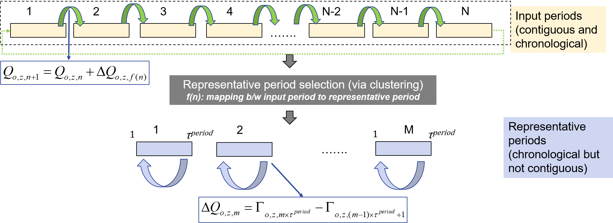Figure. Modeling inter-period energy exchange via long-duration storage when using representative period temporal resolution to approximate annual grid operations The following two equations define the storage inventory at the beginning of each input period $n+1$ as the sum of storage inventory at begining of previous input period $n$ plus change in storage inventory for that period. The latter is approximated by the change in storage inventory in the corresponding representative period, identified per the mapping $f(n)$. The second constraint relates the storage level of the last input period, $|N|$, with the storage level at the beginning of the first input period. Finally, if the input period is also a representative period, then a third constraint enforces that initial storage level estimated by the intra-period storage balance constraint should equal the initial storage level estimated from the inter-period storage balance constraints. Note that $|N|$ refers to the last modeled period.

\[\begin{aligned} & Q_{o,z,n+1} = Q_{o,z,n} + \Delta Q_{o,z,f(n)} \quad \forall o \in \mathcal{O}^{LDES}, z \in \mathcal{Z}, n \in \mathcal{N}\setminus\{|N|\} \end{aligned}\]

\[\begin{aligned} & Q_{o,z,1} = Q_{o,z,|N|} + \Delta Q_{o,z,f(|N|)} \quad \forall o \in \mathcal{O}^{LDES}, z \in \mathcal{Z}, n = |N| \end{aligned}\]

\[\begin{aligned} & Q_{o,z,n} =\Gamma_{o,z,f(n)\times \tau^{period}} - \Delta Q_{o,z,m} \quad \forall o \in \mathcal{O}^{LDES}, z \in \mathcal{Z}, n \in \mathcal{N}^{rep}, \end{aligned}\]

Finally, the next constraint enforces that the initial storage level for each input period $n$ must be less than the installed energy capacity limit. This constraint ensures that installed energy storage capacity is consistent with the state of charge during both the operational time periods $t$ during each sample period $m$ as well as at the start of each chronologically ordered input period $n$ in the full annual time series.

\[\begin{aligned} Q_{o,z,n} \leq \Delta^{total, energy}_{o,z} \quad \forall n \in \mathcal{N}, o \in \mathcal{O}^{LDES} \end{aligned}\]